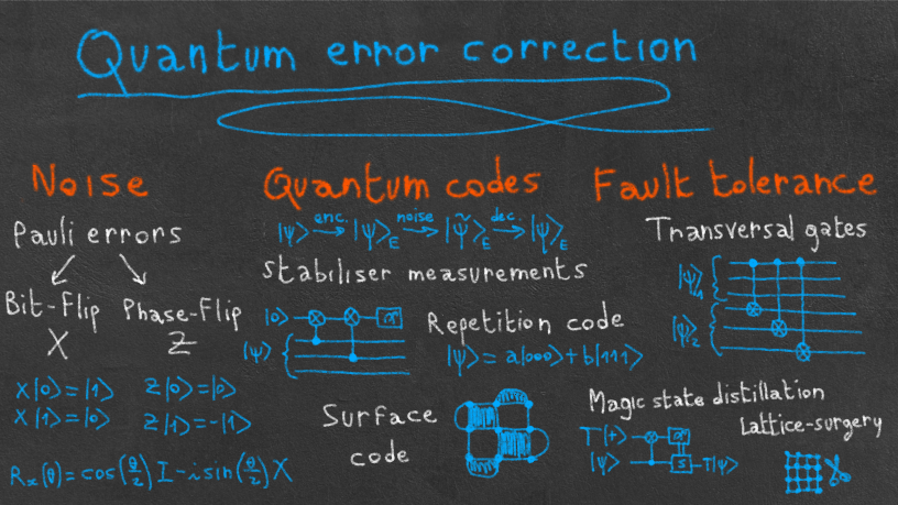
A bird's-eye view of quantum error correction and fault tolerance
This Summer marked the beginning of my thesis work, and with it, of my trip in the fascinating world of quantum error correction. I quickly found in this area the interdisciplinarity that I love: the field takes its roots in theoretical computer science (classical error correction), uses intuitions and techniques from theoretical physics (condensed matter, statistical physics, quantum field theory) and has deep connections to black hole research, statistical inference, algebraic topology and geometry, and many other areas of science and mathematics.
As I am just starting my PhD adventure, I have taken the resolution to start blogging again. And since my first task as a new PhD student is to learn as much as I can about my field, why not sharing this learning journey with you?
In this first article, we will dive together into the basics of quantum error correction (QEC). The goal is for a reader beginning in the field to get familiar with the big picture of fault-tolerance and error correction. No previous QEC background is required, but some familiarity with the basics of quantum computing (qubits, gates, measurements, etc.) is assumed.
A bit of history
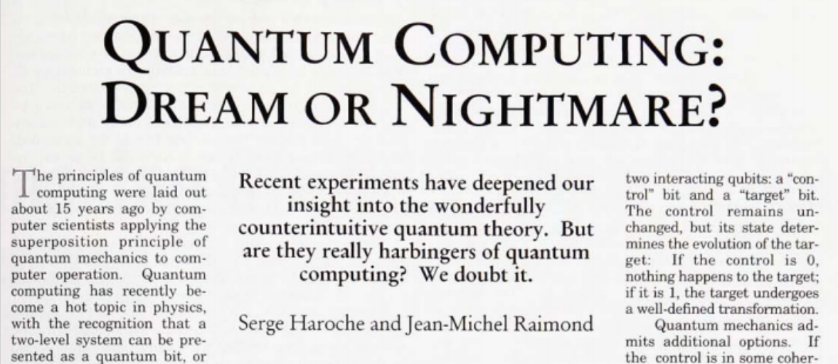
When the concept of a quantum computer was first proposed and formalized in the 1980s and 1990s, many physicists were skeptical that those devices would one day see the light of day. As an example, Serge Haroche and Jean-Michel Raimond—two eminent atomic physicists—famously said in a 1996 article in Physics Today that
The large-scale quantum machine, though it may be the computer scientist’s dream, is the experimenter’s nightmare.
The reason for their skepticism was the inherent fragility of quantum states: any noise present in a quantum system, due for instance to unwanted interactions with the environment, can irreversibly modify your quantum state.
Fortunately, the problem of computing with noise had been known for decades in the classical computing community. In the 1940s and 1950s, most computers were built from either mechanical relays or vacuum tubes, both of which were very prone to failure. It meant that random bits could flip in the middle of your calculations, giving you rubbish at the end. It’s exactly in this context that the Bell Labs mathematician Richard Hamming invented the first practical error-correcting code, out of frustration that his calculations on Model 5—a relay computer only available to him on weekends—were failing weeks after weeks1. Modern computers can still have errors from time to time (for instance due to cosmic rays!) and some critical systems therefore still require some sort of error correction. But more commonly, error-correcting codes are used everywhere in wireless communication, including satellite communication and the 4G/5G protocol.
However, generalizing those ideas from classical to quantum bits was not an easy task. The invention of the first quantum error-correcting codes, and with them of the threshold theorem, changed the game. This theorem states that there exist some families of quantum codes that can correct arbitrary errors by increasing the number of redundant qubits, as long as the noise level of the system is below a certain threshold. So, let’s say you found a code with a threshold of \(1\%\). Then, if your noise is above \(1\%\), adding more qubits to your code will yield more errors, while if it is below, adding more qubits will reduce the number of errors. The presence of a threshold below \(50\%\) is a purely quantum phenomenon: classical codes are always improved by increasing the number of redundant bits. This important difference is due to the fact that there is only one type of classical errors, the bit-flips, while quantum errors can be caused by both bit-flips and phase-flips, as we will see in the next section.
While the first quantum codes served as a useful proof of concept, their threshold was estimated to be around \(10^{-6}\), which was far below the experimental capabilities of the time 2. The introduction of the stabilizer formalism in 1998 revolutionized quantum error-correction and led to the invention of the surface code3, which has a threshold over \(1\%\) in realistic settings4. While subsequent years saw the development of many quantum codes, the surface code has remained one of the most promising one, and I will probably dedicate several articles to it. But for now, let’s try to understand how quantum error correction works.
What is quantum error correction?
Modeling quantum noise
Imagine that you are running a circuit on a real quantum computer. At each step of the circuit, you are expecting a certain state \(\vert \psi \rangle\) to come out of the device. However, if you are reading this in the 2020s, chances are that your device is noisy: instead of getting \(\vert \psi\rangle\), you will get a different state \(\vert \widetilde{\psi} \rangle\). This failure can be caused by multiple phenomena: unwanted interactions between qubits when applying a gate, unwanted interactions with the environment (causing decoherence), badly-controlled gates, errors in the measurement or state preparation process, etc. While the source of noise is diverse, it happens that a very general and simple noise model can be used to accurately model noise in a large range of situations: the Pauli error model. It consists in assuming that a Pauli operator \(X\) or \(Z\) is randomly applied after each gate or each clock cycle of the quantum computer. The generality of this model comes from the fact that any continuous error can be decomposed in the Pauli basis, and \(Y=iXZ\). For instance, if your error is an unwanted rotation by an angle \(\theta\) in the Bloch sphere (let’s say in the \(x\) direction), we can write:
\[\begin{aligned} R_x(\theta) = \cos\left(\frac{\theta}{2}\right) I - i \sin\left(\frac{\theta}{2}\right) X \end{aligned}\]implying that
\[\begin{aligned} \vert \widetilde{\psi} \rangle = R_x(\theta) \vert \psi\rangle = \cos\left(\frac{\theta}{2}\right) \vert \psi\rangle - i \sin\left(\frac{\theta}{2}\right) X \vert \psi\rangle \end{aligned}\]You will soon learn that quantum error correction is done by constantly applying non-destructive measurements to our state (the so-called stabilizer measurements), resulting in the above state being projected in either \(\vert \psi\rangle\) with probability \(\cos^2(\theta/2)\), or \(X \vert \psi\rangle\) with probability \(\sin^2(\theta/2)\). This process of decomposing any continuous error into \(X\) and \(Z\) errors is called the digitization of errors, and is key to quantum error correction, since analog errors, even on a classical computer, cannot easily be error-corrected.
So we’ve reduced the infinite range of possible continuous errors to only two types of errors: \(X\) and \(Z\). But what is the effect of those errors? Let’s consider a general single-qubit state, given by
\[\begin{aligned} \vert \psi \rangle = a \vert 0 \rangle + b \vert 1 \rangle \end{aligned}\]Applying \(X\) to it results in the state
\[\begin{aligned} X \vert \psi \rangle = a \vert 1 \rangle + b \vert 0 \rangle \end{aligned}\]In other words, we have applied a bit-flip to our state. On the other hand, applying a \(Z\) error
\[\begin{aligned} Z \vert \psi \rangle = a \vert 0 \rangle - b \vert 1 \rangle \end{aligned}\]results in a phase-flip. That’s a first major difference between classical and quantum error-correction: instead of having just one type of error (bit-flips), we now have two types of error (bit-flips and phase-flips). This is a key fact that makes classical error correction techniques not directly applicable to the quantum setting. So, how can we correct quantum errors?
Encoding and decoding
The idea of quantum error correction is to encode your state on a larger system, using redundant qubits. A simple example of encoding is the 3-repetition code, defined with the following dictionary:
\[\begin{aligned} \vert 0 \rangle \longrightarrow \vert 000 \rangle_E \\ \vert 1 \rangle \longrightarrow \vert 111 \rangle_E \end{aligned}\]It means that a general qubit \(\vert \psi \rangle = a \vert 0 \rangle + b \vert 1 \rangle\) will be encoded as \(\vert \psi \rangle_E = a \vert 000 \rangle + b \vert 111 \rangle\). We say that the code maps three physical qubits into one logical qubit.
When this encoded state goes through a noisy channel, errors can happen. But this time, we have some degree of protection. For instance, let’s say that a bit-flip occurred on the first qubit, leading to the state \(\vert \widetilde{\psi} \rangle_E = a \vert 100 \rangle + b \vert 011 \rangle\). We can then detect and correct this error, in the so-called decoding process: we perform measurements to the state and apply some correction operators depending on the measurement results. However, here comes another specificity of the quantum setting: we cannot simply measure the whole state (and then apply a majority vote or something), as it would result in a general collapse of the state. So we need to apply non-destructive measurements, also called stabilizer measurements. An example of stabilizer measurement would be to measure the parity of each pair of qubits, i.e. whether the two qubits are equal or not. For instance, the following circuit can be used to measure the parity of qubits 1 and 2:
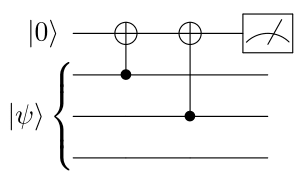
Indeed, if the first two qubits are in the state \(\vert 00 \rangle\) or \(\vert 11 \rangle\), you can check that the measurement result in the \(Z\) basis will be \(1\) (i.e. the ancilla qubit is in the \(\vert 0 \rangle\) state), while if we are in either \(\vert 01 \rangle\) or \(\vert 10 \rangle\), the measurement result will be \(-1\). Note that by measuring the ancilla qubit, our state has not been destroyed.
So, what happens if we apply those parity measurements to the state \(\vert \widetilde{\psi} \rangle_E = a \vert 100 \rangle + b \vert 011 \rangle\)? We will see that qubits 2 and 3 are equal, while qubit 1 is different from the two others. Assuming that we only had one \(X\) error, we can deduce that the only possibility is that the first qubit has been subjected to a bit-flip. Therefore, we apply a Pauli \(\text{X}\) operator on the first qubit to recover our original state.
The quantum error-correction process can be summarized by the following diagram:
\[\begin{aligned} \vert \psi \rangle \xrightarrow{\text{encoding}} \vert \psi \rangle_E \xrightarrow{\text{noise}} \vert \widetilde{\psi} \rangle_E \xrightarrow{\text{decoding}} \vert \psi \rangle_E \end{aligned}\]Note that our code has two major drawbacks: it cannot correctly decode more than one bit-flip errors, and cannot detect phase-flip errors at all. While the first problem could be alleviated by increasing the number of physical qubits, the second one is more fundamental and requires the design of more complex quantum codes. One of the most popular such code is the surface code (also called toric code), which belongs to the more general class of topological quantum codes.
Surface code
Explaining exactly how the surface code work is a out-of-scope for this article, as it would require a proper introduction to the stabilizer formalism. However, given the importance this code has taken in the QEC world, I couldn’t resist giving you a big picture overview of its main characteristics, as a treat before I write a dedicated article on the topic! If you want to get a more in-depth explanation, feel free to look at the resources posted at the end of this article, such as this series of blog post by James Wootton!
So what is the surface code? It’s a code that encodes one logical qubit on a 2D grid of \(L^2\) physical qubits. For instance, the picture below represents one logical qubit of the surface code, encoded with 25 physical qubits (the white dots). The two colors represent the two types of measurements that are used to detect errors, made either of \(X\) operators (to detect phase-flips) or \(Z\) operators (to detect bit-flips), but we won’t dive into those details now.
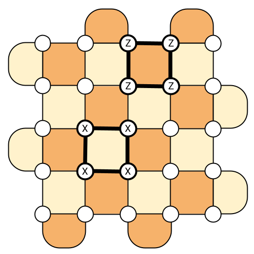
To achieve noise levels that are low enough to run something like Shor’s algorithm might require grids containing between 1,000 and 10,000 physical qubits per logical qubit5! While it might sound like a huge overhead (and indeed, it is!), the surface code still has a few advantages, otherwise it wouldn’t be the most popular code in the market! First, contrary to the repetition code that we saw in the previous section, it can detect both bit-flips and phase-flips. Since doing so is one of the main difficulties in designing QEC codes and the reason why we cannot simply generalize classical codes, it is worth noting. A second advantage compared to other QEC codes is that it’s two-dimensional. It means that in practice, we only need to arrange the qubits on a physical 2D chip with interaction between nearest neighbors, which makes the surface code particularly promising for superconducting chips like IBM’s and Google’s quantum computers. Finally, the threshold has been calculated to be around \(\sim 1\%\) (the exact number depends on the exact nature of the noise), which is one of the highest in the QEC zoo5. As a reminder, the threshold is the noise level below which increasing the number of physical qubits (here the size of the grid) actually improves the number of errors that can be corrected. So to make the surface code work, it means that we just need our noise level to be below \(1\%\) (probably slightly lower in realistic settings), which is definitely within the range of what experimentalists can do!
Note that many alternatives to the 2D surface code have been proposed, such as 3D and 4D surface codes, color codes, low-density parity-check codes (also known as LDPC codes), subsystem codes, etc. Choosing a code is often a trade-off between connectivity (e.g. LDPC codes often require long-range interaction, so are not easily implementable on 2D chips), ease of measurements (how many qubits are measured simultaneously to detect errors), performance with a given noise model, threshold, gate design, etc.
Once the encoding and decoding procedures are established, there is still one last step before being able to do quantum computation error-free: designing logical gates that act on the code. It happens that this task is far from trivial in general, and a whole subfield of QEC is dedicated to it. That’s the subject of fault-tolerant quantum computing.
Fault-tolerant quantum computing
Transversality and fault-tolerance
The main challenge in designing gates is to avoid the propagation of errors: if we’re not careful, multi-qubit gates can turn one-qubit errors into correlated multi-qubit ones. This is particularly disturbing when the gate couples several physical qubits representing a single logical one (what we call a block). For instance, imagine you want to apply a logical Hadamard on the 3-repetition code considered earlier. This gate, that we can call \(H_L\), should use three physical qubits to act on one logical qubit, i.e.:
\[\begin{aligned} H \vert 0 \rangle = \frac{1}{\sqrt{2}} \left( \vert 0 \rangle + \vert 1 \rangle \right) \; \xrightarrow{\text{encoding}} \; H_L \vert 000 \rangle = \frac{1}{\sqrt{2}} \left( \vert 000 \rangle + \vert 111 \rangle \right) \\ H \vert 1 \rangle = \frac{1}{\sqrt{2}} \left( \vert 0 \rangle - \vert 1 \rangle \right) \; \xrightarrow{\text{encoding}} \; H_L \vert 111 \rangle = \frac{1}{\sqrt{2}} \left( \vert 000 \rangle - \vert 111 \rangle \right) \end{aligned}\]To implement the unitary \(H_L\), some entangling gates will be needed. For example, you can check that the following circuit gives the correct unitary on \(\vert 000 \rangle\) and \(\vert 111 \rangle\):
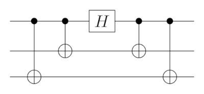
The issue here is the presence of physical CNOTs within the block, as they can create correlated errors that won’t be easily correctable.
On the other hand, if we wanted to implement a logical CNOT between two logical qubits \(\vert \psi \rangle_1\) and \(\vert \psi \rangle_2\), we would simply use the following circuit
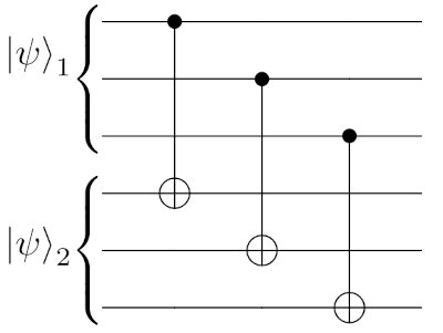
which doesn’t contain any entangling gate within each block. Such gate is called transversal, while the Hadamard gate we saw previously was non-transversal. An encoded circuit composed only of transversal gates is fault-tolerant, meaning that it doesn’t propagate errors further.
So, do we know any code such that all the gates can be built transversally? Unfortunately, the answer is no, and we even know that such code cannot exist. That’s the object of a foundational theorem in the field, called the Eastin-Knill theorem, which states that for any QEC code, there is no universal gate set6 made only of transversal gates. For instance, in the surface code, only Clifford gates can be implemented transversally, i.e. all the gates that can be constructed from \(H\), \(CNOT\) and \(S\) gates. It includes all Pauli gates, but not the \(T\) gate for example, which is required for universality.
Magic state distillation
Many tricks have been proposed to “by-pass” this no-go theorem. One of the most common tricks is called magic state distillation. To illustrate how it works, let’s say we want to implement a \(T\) gate fault-tolerantly. As a reminder, the \(T\) gate is a one-qubit gate defined by the matrix
\[\begin{aligned} T = \left( \begin{matrix} 1 & 0 \\ 0 & e^{i\pi/4} \\ \end{matrix} \right) \end{aligned}\]and is one of the simplest examples of non-Clifford gate, meaning that it cannot be written out of just \(H\), \(S\) and \(CNOT\). On the other hand, appending it to the Clifford gate set leads to a universal gate set, i.e. any gate you can think of can be written out of just \(T\), \(H\) and \(CNOT\) (we don’t need \(S\) anymore, since \(S=T^2\)). Since the surface code can already implement all Clifford gates fault-tolerantly, it means that we only need a procedure to implement \(T\) gates!
The first idea of magic state distillation is to implement the state \(T\vert+\rangle=\vert 0 \rangle + e^{i\pi/4} \vert 1 \rangle\) non-fault-tolerantly on an ancilla qubit (meaning that errors can occur when creating the state) and to “inject” it in the qubits of our code, thereby creating a \(T\) gate on those qubits. This trick, called state injection (or gate teleportation in the measurement-based QC community) can be summarized by the following circuit:
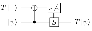
where the \(S\) gate is applied when the measurement of the ancilla qubit leads \(1\). It’s a little exercise the check that the circuit above indeed leads to a \(T\) gate (and you can find the answer on Stack Exchange). The state \(T\vert + \rangle\) is called a magic state, and as we saw, its preparation can involve some errors (it’s not fault-tolerant). The second idea of magic state distillation is therefore distillation. By preparing \(N\) copies of a noisy magic state, it’s possible to create an arbitrary clean \(T\) gate (similarly to how entanglement distillation is done in quantum communication). The full protocol can be shown to be fault-tolerant, but it often requires a very large overhead in both the number of qubits and number of gates7. This overhead led to the claim that obtaining a quantum advantage with quadratic speed-ups might be unrealistic in the first fault-tolerant quantum computers8. Reducing this overhead or finding codes that don’t need magic state distillation is therefore a very important research problem.
Measurement-based gates: lattice surgery and twists
So far, we have presented transversal gates as the good guys of fault-tolerant quantum computing, as they can be implemented directly without propagating errors. However, transversal two-qubit gates, while fault-tolerant, are often far from practical. Take two logical qubits of the surface code for instance, and align them on a single 2D lattice.
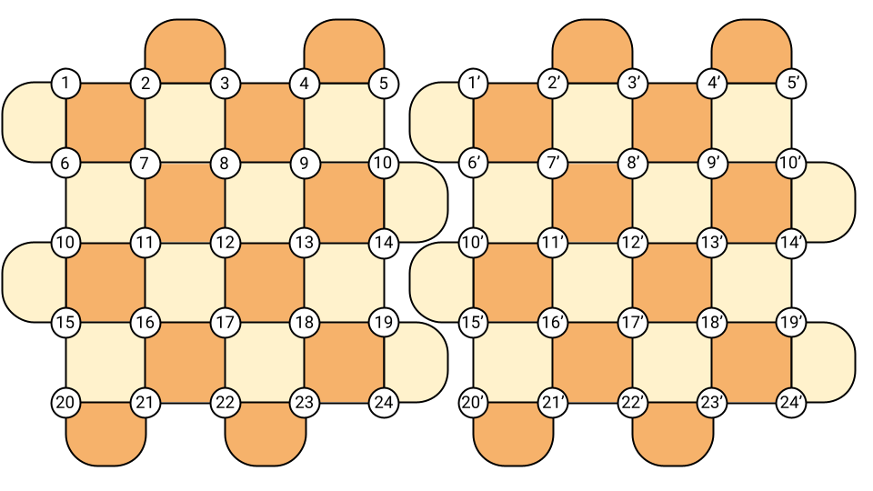
A transversal two-qubit gate would consist in \(L^2\) physical gates between each pair of qubits \(a\) and \(a'\). However, as seen in the picture above, it would require some long-range interactions, since qubits \(a\) and \(a'\) are always \(L\) qubits apart. A solution could consist in putting one surface code above the other (in 3D). However, 3D chips are hard to build in practice, and it happens that more convenient solutions exist, namely lattice surgery and twist deformations.
In both methods, gates are applied by performing measurements and temporarily changing the code itself. In lattice surgery, those measurements allow merging different surface codes into a single one, and split it again when needed. It can be shown that many gates, such as the CNOT gate, can be designed by performing such a series of merge and split operations. In twist deformations, measurements create holes in the lattice, and braiding operators around those holes allow to create some gates. All those operations are local, making both techniques amenable to real devices. I hope to describe those techniques in more details in future posts.
Measurement errors
Finally, in fault-tolerant quantum computing, the measurement apparatus is also crucial. To detect errors, measurements are made all the time, and those can be very noisy. It means that our stabilizer measurements can lead to the wrong answer. To mitigate this effect, the basic technique simply consists in repeating the stabilizer measurements many times. However, some codes such as the 3D surface code have a property that make them amenable to single-shot quantum error correction, as set of techniques that allow to correct errors with a single noisy measurement per stabilizer. More generally, any fault-tolerant scheme must also include a method to perform measurements without propagating errors in a non-fault-tolerant way.
Conclusion
In this first post, we set eyes on the big picture of QEC and its different subfields. We discussed a lot of notions and introduced a lot of jargon, that we will review in detail in different posts, so don’t worry if a few things are unclear for the moment. Just retain that quantum error correction comprises two main challenges: designing an encoding process that can protect qubits against noise, and building actual circuits on the code without introducing more errors (the subject of fault-tolerance). In the meantime, feel free to use the following resources if you want to learn more about any of those topics.
Resources
- Quantum Error Correction: An Introductory Guide, by Joschka Roffe
- Lectures on Topological Codes and Quantum Computation, by Dan Browne
- Video lectures on Quantum Error Correction and Fault Tolerance, by Daniel Gottesman
- Quantum Computation and Quantum Information — Chapter 7, Nielsen & Chuang
- What is Quantum Error Correction, series of blog posts by James Wootton
-
Richard Hamming, The Art of Doing Science and Engineering, 1997 ↩︎
-
E. Knill, R. Laflamme, W. Zurek, Threshold Accuracy for Quantum Computation, 1996 ↩︎
-
Eric Dennis, Alexei Kitaev, Andrew Landahl, John Preskill, Topological quantum memory, 2001 ↩︎
-
David S. Wang, Austin G. Fowler, Lloyd C. L. Hollenberg, Quantum computing with nearest neighbor interactions and error rates over 1%, 2010 ↩︎
-
Austin G. Fowler, Matteo Mariantoni, John M. Martinis, Andrew N. Cleland, Surface codes: Towards practical large-scale quantum computation ↩︎ ↩︎2
-
Here, a universal gate set is defined as a set that can approximate any unitary up to a precision \(\epsilon\) with \(O\left(\log\left( \frac{1}{\epsilon}\right)^c\right)\) gates. ↩︎
-
Sergey Bravyi, Jeongwan Haah, Magic-state distillation with low overhead ↩︎
-
Ryan Babbush, Jarrod McClean, Michael Newman, Craig Gidney, Sergio Boixo, Hartmut Neven, Focus beyond quadratic speedups for error-corrected quantum advantage ↩︎