All you need to know about classical error correction

21 May 2022 on Quantum Computing

When learning about quantum error correction (QEC) for the first time, I tried to jump directly into the core of the subject, going from the stabilizer formalism to topological codes and decoders, but completely missing the classical origin of those notions. The reason is that many introductions to the subject do a great job presenting all those concepts in a self-contained way, without assuming any knowledge in error correction. So why bother learning classical error correction at all? Because if you dig deeper, you will find classical error correction concepts sprinkled all over QEC. Important classical notions such as parity checks, linear codes, Tanner graphs, belief propagation, low-density parity-check (LDPC) codes and many more, have natural generalizations in the quantum world and have been widely used in the development of QEC. Learning about classical error correction a few months into my QEC journey was completely illuminating: many ideas that I only understood formally suddenly made sense intuitively, and I was able to understand the content of many more papers. For this reason, I’d like this second article on quantum error correction to actually be about classical error correction. You will learn all you need to start off your QEC journey on the right foot!

So what exactly are we gonna study today? The central notion in this post is that of linear code. Linear codes form one of the most important families of error-correcting codes. It includes for instance Hamming codes (some of the earliest codes, invented in 1950), Reed-Solomon codes (used in CDs and QR codes), Turbo codes (used in 3G/4G communication) and LDPC codes (used in 5G communication). While we won’t try to cover the whole zoo of linear codes here, we will introduce some crucial tools to understand them. In particular, the goal of this post is to give you a good grasp of the parity-check matrix, and its graphical representation, the Tanner graph. As we will see when going quantum, the stabilizer formalism (the dominant paradigm to construct quantum codes) can be understood as a direct generalization of linear coding theory, and the quantum parity-check matrix happens to be an essential tool to simulate quantum codes in practice. This post will also be the occasion to introduce some more general coding terminology (encoding, decoding, distance, $[n,k,d]$-code, codewords, etc.), which will be handy when delving into QEC.

As a final motivating factor before starting, it happens that this field contains some of the most beautiful ideas in computer science. To get a sense of this beauty, I recommend watching the 3Blue1Brown videos on the Hamming code as a complement to this post. It will give you a very visual picture of some of the techniques introduced here. However, it’s not a prerequisite, so feel free to continue reading this post and watch the video at a later time. On that note, let’s start!

General setting

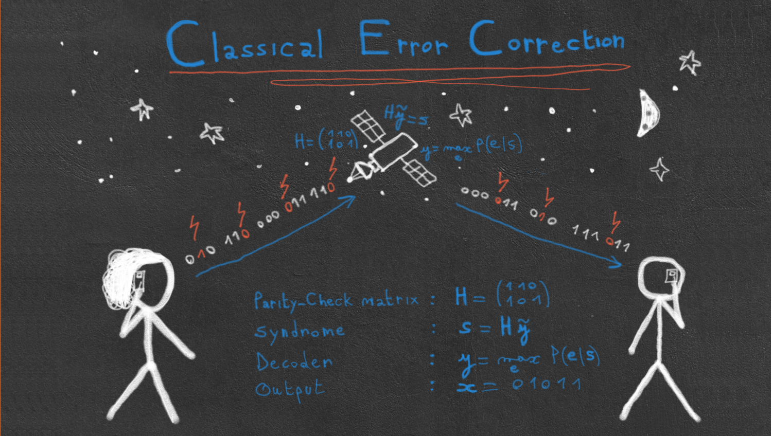
Let us consider the following setting: we would like to send a $k$-bit message $\bm{x}$ across a noisy channel, for instance between your phone and a satellite. If we choose to send $\bm{x}$ directly without any pre-processing, a different result $\widetilde{\bm{x}}$ will arrive with a certain number of errors. Here, we will assume that all errors are bit-flip errors, meaning that they can turn a $1$ into $0$ or a $0$ into $1$ (potentially with a different probability).

To protect the message against bit-flip errors, we can choose to add redundancy to it. For instance, let’s send all the bits three times: each $0$ becomes $000$ and each $1$ becomes $111$. For example, if we want to send the message $10100$, we should send instead

$$\begin{aligned} 111,000,111,000,000 \end{aligned}$$

Now, imagine some errors have occurred, and the satellite receives the following message instead:

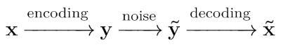
$$\begin{aligned} 101,000,111,000,100 \end{aligned}$$

Assuming that at most one error has occurred on each triplet, the original message can be decoded by taking a majority vote: $101$ is decoded as $1$ and $100$ is decoded as $0$. The message $\bm{y}=\bm{x} \bm{x} \bm{x}$ that we send across the channel is called an encoding of $\bm{x}$, while trying to infer the original message $\bm{x}$ from the noisy encoding $\bm{\tilde{y}}$ is called decoding. A particular encoding is often called a code as well, and the example we have seen is called the 3-repetition code. More generally, an error-correction process can be summarized with the following diagram:

Let’s now introduce some important jargon. In general, an encoder $\mathcal{E}$ divides a message into chunks of $k$ bits, and encodes them into $n$ bits. We write $\mathcal{E}(\bm{x})=\bm{y}$, where $\bm{x}$ is a $k$-bit message and $\bm{y}$ is an $n$-bit encoding. For example, in the 3-repetition code, we are encoding one bit at a time into three bits, so $k=1$, $n=3$, and $\mathcal{E}(x)=xxx$ for each bit $x$.

A codeword is an element of the image of $\mathcal{E}$. We denote the set of all codewords as $\mathcal{C}=\text{Im}(\mathcal{E})$. For instance, in the 3-repetition code, we have two codewords: $000$ and $111$, respectively given by $\mathcal{E}(0)$ and $\mathcal{E}(1)$. In this example, we see that if one or two errors occur on a given codeword, the resulting bit-string won’t be a codeword anymore, making the error detectable. For instance, if you see $110$ in your message, you know that an error has occurred, since $110$ is not a codeword. On the other hands, the error will only be correctable by our majority vote procedure if at most one error occurs. Finally, if three bit-flips occur—going from $000$ to $111$ or the reverse—, the errors will be undetectable, resulting in what we call a logical error.

This argument can be generalized using the notion of distance. The distance $d$ of a code is the minimum number of bit-flips required to pass from one codeword to another, or in other words, the minimum number of errors that would be undetectable with our code. To define the distance more formally, we need to introduce two important notions. The Hamming weight $\vert\bm{x}\vert$ of a binary vector $\bm{x}$ is the number of $1$ of this vector. The Hamming distance $D_H(\bm{x},\bm{y})$ between two binary vectors $\bm{x}$ and $\bm{y}$ is the number of components that differ between $\bm{x}$ and $\bm{y}$, i.e.

$$\begin{aligned} D_H(\bm{x},\bm{y})=\vert \bm{x} - \bm{y} \vert \end{aligned}$$

We can then define the distance as the minimum Hamming distance between two vectors:

$$\begin{aligned} d=\min_{\bm{x},\bm{y} \in \mathcal{C}} D_H(\bm{x},\bm{y}) \end{aligned}$$

For instance, the distance of the 3-repetition code is 3 (we need to flip all 3 bits to have an undetectable error). A code that encodes $k$ bits with $n$ bits and has a distance $d$ is called an $[n,k,d]$-code. The 3-repetition code is an example of $[3,1,3]$-code.

Finally, the rate of an $[n, k, d]$-code is defined as $R=k/n$ (so $R=1/3$ in our case).

The difficulty in designing good error-correcting codes lies in the trade-off between rate and distance. Indeed, we would ideally like both quantities to be high: a high rate means that there is a low overhead in the encoding process (we only need a few redundancy bits), and a high distance means that we can correct many errors. So can we maximize both quantities? Unfortunately, many bounds have been established on this trade-off, telling us that high-rate codes must have low distance, and high-distance codes must have low rate. The easiest bound to understand is the Singleton bound, which states that for any linear $[n, k, d]$-code (we will see the definition of a linear code shortly), we have

$$\begin{aligned} k \leq n - d + 1 \end{aligned}$$

or in terms of rate

$$\begin{aligned} R \leq 1 - \frac{d - 1}{n} \end{aligned}$$

This shows that we cannot arbitrarily increase the rate without decreasing the distance. We will see an interesting illustration of this trade-off in this post by introducing two codes with opposite characteristics: the Hamming code and the simplex code. While the first one is an $[n, n - \log(n+1), 3]$-code (high rate, low distance), the second one is an $[n, \log(n), n/2]$-code (low rate, high distance).

We have introduced a lot of notations and jargon in this section, which can be overwhelming when seen for the first time. That’s what happens when you decide to learn a new field! But don’t get discouraged, those notations will keep appearing all the time during your (quantum) error correction learning trip, so they will soon be very familiar to you. In the meantime, I encourage you to do the following three (short) exercises to consolidate what you’ve just learned (the solutions are at the end of the post).

Exercise 1: We define the $\ell$-repetition code as the repetition of each bit of the message $\ell$ times. Work out the encoding function $\mathcal{E}$ and the different codewords, as well the parameters $n$, $k$ and $d$ of the code. How many errors per codeword are detectable? Correctable? What is the rate of the code, and its limit when $\ell \rightarrow \infty$?

Exercise 2: Show that an $[n,k,d]$-code can detect up to $d-1$ errors and correct up to $\frac{d-1}{2}$ errors.

Exercise 3: Show that for an $[n,k,d]$-code defined by the set of codewords $\mathcal{C}$, we have $\vert\mathcal{C}\vert=2^k$.

Parity-checks and Hamming codes

In 1950, Richard Hamming discovered a more intelligent way to introduce redundancy in a message than having to repeat it several times. As a warm-up to understand his method, let’s consider the following code, called simple parity-check code, that encodes $k=3$ bits into $n=4$ bits

$$\begin{aligned} \mathcal{E}(abc) = a b c z \end{aligned}$$

where $z = a + b + c \; (\text{mod} \; 2)$. We call $z$ a parity-check bit, as it indicates whether there is an even or an odd number of $1$s in the sum ($z=0$ for even and $z=1$ for odd). As an exercise, try to write the different codewords corresponding to this encoding map!

Now, we can show that any single error can be detected by this code. Indeed, if one of the bits $a, b, c$ gets flipped, the parity of the three bits will be reversed, and we won’t have $z=a + b + c \; (\text{mod} \; 2)$ anymore, indicating that an error have occurred. Similarly, if $z$ gets flipped, it won’t correspond to the parity of $a,b,c$ anymore and we will detect an error.

However, there is no way to know where the error has occurred using this code, or in other words, errors are not correctable. The genius of Hamming was to find a way to use parity checks to actually know the position of the error!

To illustrate his method, let us consider a 4-bit message $\bm{x}=abcd$, as well as the three variables $z_1, z_2, z_3$ given by

$$\begin{aligned} z_1 &= a + b + d \\ z_2 &= a + c + d \\ z_3 &= b + c + d \\ \end{aligned}$$

where the sum is taken modulo 2 (we will consider all the sums of bits to be modulo 2 from now on, without explicitely writing $\mod 2$). Those variables indicate the parity of different chunks of our message, as illustrated here:

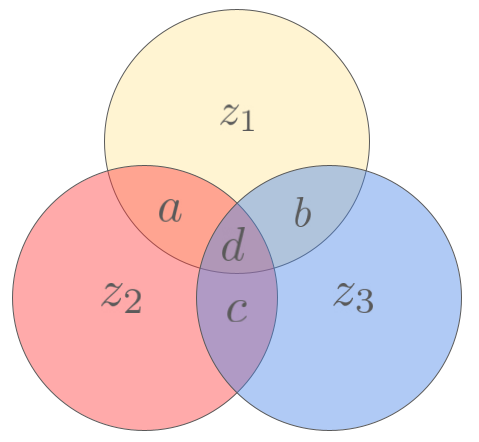
In this diagram, each circle represents a parity-check bit $z_i$, and each intersection represents a message bit $a,b,c,d$. By construction, each parity-check bit only involves the three message bits contained in its corresponding circle.

If we now send the 7-bit message $\bm{y}=\mathcal{E}(abcd)=abcdz_1z_2z_3$, we can show that any single-bit error will be correctable. Indeed, let’s see what happens if an error occurs on bit $a$. In this case, we can read in the diagram above that both $z_1$ and $z_2$ parity checks will be violated, while $z_3$ will remain equal to $b+c+d$. This can only happen if $a$ is flipped, which allows us to correct the error. A similar reasoning can be performed for the other bits. This code, called the $[7,4]$-Hamming code, is a $[7,4,3]$-code with a rate $R=4/7 \approx 0.57$, which is already better than the rate $R \approx 0.33$ of the $3$-repetition code, for the same distance.

The construction presented here can be generalized, leading to a whole family of Hamming codes defined for any $n$ of the form $n=2^r-1$. We won’t go into the details of this construction here, but if you’re interested, I encourage you to watch this 3Blue1Brown video on the topic. The main takeaway from the general Hamming code construction is that we only need a logarithmic number of parity checks to correct all single-bit errors! More precisely, Hamming codes are $[2^r-1, 2^r-r-1, 3]$-codes, with a rate $R=\frac{2^r-r-1}{2^r-1}$ that converges to $1$ when $r \rightarrow \infty$.

However, Hamming codes have a low distance that doesn’t increase with the codeword length, and they would therefore be impractical in very noisy systems. So we need a more general framework that would allow us to find new codes with better characteristics. That framework is the one of linear codes.

Linear codes

This idea of transmitting both the message and some parity-check bits can be generalized with the notion of linear code. A linear code consists in using a matrix $\bm{G}$—called generator matrix—as our code, i.e.

$$\begin{aligned} \bm{y} = \bm{G} \bm{x}. \end{aligned}$$

If our message $\bm{x}$ has length $k$ and is complemented by $m$ parity checks, such that $n=k+m$ is the size of $\bm{y}$, we can write $\bm{G}$ as

$$\begin{aligned} \bm{G}=\left(\begin{matrix} I_k \\ \hline \bm{A} \end{matrix} \right) \end{aligned}$$

with $I_k$ the $k \times k$ identity matrix (used to reproduce the message in the code) and $\bm{A}$ an $m \times k$ matrix that performs the parity checks. In this notation, all the matrix operations are performed modulo 2. For instance, the generator matrix of the Hamming code can be written

$$\begin{aligned} \bm{G} = \left( \begin{matrix} 1 & 0 & 0 & 0 \\ 0 & 1 & 0& 0 \\ 0 & 0 & 1 & 0 \\ 0 & 0 & 0 & 1 \\ \hline 1 & 1 & 0 & 1 \\ 1 & 0 & 1 & 1 \\ 0 & 1 & 1 & 1 \end{matrix} \right) \end{aligned}$$

since

$$\begin{aligned} \bm{G} \bm{x} = \left( \begin{matrix} 1 & 0 & 0 & 0 \\ 0 & 1 & 0& 0 \\ 0 & 0 & 1 & 0 \\ 0 & 0 & 0 & 1 \\ \hline 1 & 1 & 0 & 1 \\ 1 & 0 & 1 & 1 \\ 0 & 1 & 1 & 1 \end{matrix} \right) \left( \begin{matrix} a \\ b \\ c \\ d \end{matrix} \right) = \left( \begin{matrix} a \\ b \\ c \\ d \\ a + b + d \\ a + c + d \\ b + c + d \end{matrix} \right) = \left( \begin{matrix} a \\ b \\ c \\ d \\ z_1 \\ z_2 \\ z_3 \end{matrix} \right) \end{aligned}$$

Two important remarks about generator matrices:

1. Elementary operations on the rows and columns of $\bm{G}$ don’t change the code. Indeed, the code is defined as the image of $G$, which is invariant under similarity transformations. Using Gaussian reduction, it is therefore always possible to transform $\bm{G}$ to have the form $\bm{G}=\left(\begin{matrix} I_k \\ \hline \bm{A} \end{matrix} \right)$. In other words, any linear code can be seen as a message supplemented with parity checks!
2. The codewords of a code described by $\bm{G}$ can be found by taking all the linear combinations of the columns of $\bm{G}$ (the vector $\bm{x}$ in the definition indicates which columns you select or not). Therefore, to find all the codewords, just calculate all the $\bm{y}$ of the form $\bm{y}=a_1 \bm{c_1} + ... a_k \bm{c_k}$ where $\bm{c_i}$ is the $i^{\th}$ column of $G$ and $a_1,...a_k \in \{0,1\}$.

An equivalent picture to describe linear codes is through the parity-check matrix, defined as an $m \times n$ matrix $\bm{H}$ such that

$$\begin{aligned} \bm{H} \bm{y} = 0 \end{aligned}$$

if and only if $\bm{y}$ is a codeword. In other words, the space of codewords can be defined as the kernel of $\bm{H}$. The intuition is that linear codes can always be defined as a set of codewords obeying a certain system of linear equations, defined by the parity checks. For instance, the codewords of the Hamming code obey the following system:

$$\begin{aligned} a + b + d + z_1 = 0 \\ a + b + c + z_2 = 0 \\ b + c + d + z_3 = 0 \end{aligned}$$

(since $a+b+d=z_1 \Leftrightarrow a+b+d+z_1=0$ when working modulo $2$)

Therefore, the parity-check matrix of the Hamming code can be written

$$\begin{aligned} \bm{H} = \left( \begin{array}{cccc|ccc} 1 & 1 & 0 & 1 & 1 & 0 & 0 \\ 1 & 0 & 1 & 1 & 0 & 1 & 0 \\ 0 & 1 & 1 & 1 & 0 & 0 & 1 \\ \end{array} \right) \end{aligned}$$

For a generator matrix of the form $\bm{G}=\left(\begin{matrix} I_k \\ \hline \bm{A} \end{matrix} \right)$, the corresponding parity-check matrix can be written

$$\begin{aligned} \bm{H}=\left(\begin{matrix} \bm{A} & I_m \end{matrix} \right) \end{aligned}$$

Indeed, if $\bm{y}$ is a codeword, it can be written $\bm{y}=\bm{G}\bm{x}=\left(\begin{matrix} \bm{x} \\ \hline \bm{A} \bm{x} \end{matrix} \right)$. Applying $\bm{H}$, we get

$$\begin{aligned} \bm{H} \bm{y} = \bm{A}\bm{x} + \bm{A}\bm{x} = 2\bm{A}\bm{x} = \bm{0} \end{aligned}$$

since all operations are performed modulo 2, and $2=0 \mod 2$.

Similarly to how all generator matrices can be chosen to have the form $\bm{G}=\left(\begin{matrix} I_k \\ \hline \bm{A} \end{matrix} \right)$, we can always apply a Gaussian reduction on $H$ such that is has the form $\bm{H}=\left(\begin{matrix} \bm{A} & I_m \end{matrix} \right)$.

At this point of the post, you might be wondering why we should use the parity-check matrix, when the generator matrix seems much more natural. There are many reasons to prefer the parity-check matrix over the generator matrix. The simplest one is that it gives a convenient method to detect and correct errors. Indeed, if $\widetilde{\bm{y}}=\bm{y} + \bm{e}$ is the received message disturbed by an error vector $\bm{e}$, applying the parity-check matrix to $\widetilde{\bm{y}}$ gives

$$\begin{aligned} \bm{H} \widetilde{\bm{y}} &= \bm{H} \left( \bm{y} + \bm{e} \right) \\ &= \bm{H} \bm{e} \end{aligned}$$

The new vector $\bm{s} = \bm{H} \bm{e}$ has dimension $m$ and is called the syndrome. Each component $s_i$ of the syndrome is equal to $1$ if the parity-check equation $i$ is violated. Decoding a message then consists in finding the most probable error $\bm{e}$ that has yielded to the syndrome $\bm{s}$. Let’s illustrate this syndrome decoding technique with the $[7,4]$-Hamming code. The components of the syndrome are given by the following system of equations:

$$\begin{aligned} a + b + d + z_1 = s_1 \\ a + b + c + z_2 = s_2 \\ b + c + d + z_3 = s_3 \end{aligned}$$

When $s_i=1$, it therefore means that the parity-check bit $z_i$ is violated (it doesn’t correspond to the parity of its block anymore). The following table shows the bit we choose to correct for each of the 8 possible syndromes (we can obtain it by looking at the Venn diagram of the Hamming code):

Syndrome	000	001	010	011	100	101	110	111
Correction	$\emptyset$	$z_1$	$z_2$	$c$	$z_3$	$b$	$a$	$d$

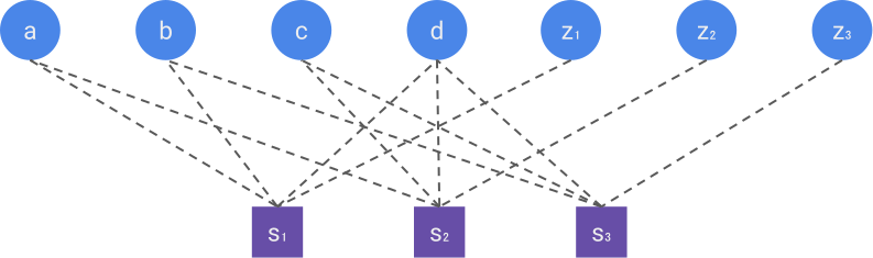
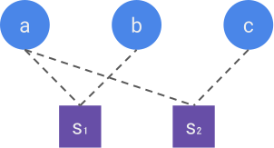
A visual way to construct the parity-check matrix is through the Tanner graph of the code. The Tanner graph is a bipartite graph containing two types of nodes, the data nodes (one for each bit of the codeword) and the check nodes (one for each bit of the syndrome). A check node $i$ and a data node $j$ are connected if the syndrome bit $s_i$ depends on $x_j$. The figure below represents the Tanner graph of the Hamming code. The parity-check matrix is then simply the adjacency matrix of the Tanner graph, i.e. it has a $1$ at row $i$ and column $j$ if the check node $i$ is connected to the data node $j$, and $0$ otherwise.

Tanner graph of the Hamming code. The top nodes represent the codeword bits and the bottom nodes the syndrome bits, with an edge whenever a codeword bit is involved in the definition of a syndrome bit.

In quantum error correction, the syndrome can be measured without disturbing the state (through the so-called stabilizer measurements), which makes the theory of linear codes easily transferable to the quantum domain. While quantum codewords can be complicated superpositions in the Hilbert space, errors are simple vectors of size $n$ (the number of qubits), making the calculation of the syndrome $\bm{s}=\bm{H} \bm{e}$ straightforward using the the parity-check matrix, and it is indeed used extensively in simulations.

In the next section, we will study the problem of decoding linear codes in general, i.e. correcting the errors using the syndrome information. But before that, you can try to solve the following exercises to make sure you understand the basics of linear codes.

Exercise 4: Find the generator and the parity-check matrix of the code defined by $\mathcal{E}(abc) = a b c z$ where $z=a+b+c$, and draw its Tanner graph.

Exercise 5: Find the generator and the parity-check matrix of the 3-repetition code, and draw its Tanner graph.

Exercise 6: Show that the set of codewords is a vector space, i.e. if two vectors $\bm{y_1}$ and $\bm{y_2}$ are codewords, $\bm{y_1} + \bm{y_2}$ is also a codeword. This property is sometimes taken as the definition of linear codes.

Exercise 7: (a) Show that if $V$ is a vector space over binary numbers, then $\vert V\vert = 2^{\dim(V)}$, where $\vert V\vert$ is the the number of elements in the vector space. $\newline$ (b) Deduce that the parity-check matrix $\bm{H}$ of an $[n,k,d]$-code obeys the relation $\text{rank}(H)=n-k$.$\newline$ (c) Deduce that if a code has $m$ independent parity checks, we have $m=n-k$. This relation is often used to find the parameter $k$ of a code given the parity checks.

Exercise 8: (a) Show that the distance of a linear code is the minimum Hamming weight of all the non-zero codewords, i.e. $d=\min_{\bm{y}\in \mathcal{C}, \bm{y} \neq \bm{0}} \vert \bm{y} \vert$, where $\mathcal{C}$ is the space of codewords and $\vert\cdot\vert$ denotes the Hamming weight (Hint: first prove that the Hamming distance between two codewords is translation-invariant, i.e. $D_H(\bm{x},\bm{y})=D_H(\bm{x}+\bm{z},\bm{y}+\bm{z})$)$\newline$ (b) Use this property to compute the distance of the Hamming code.

Decoding linear codes

Designing a code with good characteristics, such as a high rate and a high distance, is not enough to make it practical: you need to show how to decode it efficiently. As discussed before, decoding consists in finding the original message given its noisy encoded version. We then define an efficient decoder as an algorithm able to accomplish this task in polynomial time, i.e. with a time complexity that grows polynomially with the size $n$ of the code.

To see why decoding can be a difficult problem, let’s consider the general task of decoding a linear code, when errors follow a certain distribution $P(\bm{e})$. As we’ve seen in the previous section, decoding a linear code can be reduced to finding the most likely error given a received syndrome. Let $\bm{H}$ denote the parity-check matrix of our code and $\bm{s}=\bm{H}\bm{e}$ the received syndrome . The goal of an ideal decoder would be to find the vector $\bm{e}$ that maximizes the probability $P(\bm{e} \vert \bm{s})$. Using Bayes rule, we can write this probability as:

$$\begin{aligned} P(\bm{e} \vert \bm{s}) = \frac{P(\bm{s} \vert \bm{e}) P(\bm{e})}{P(\bm{s})} \end{aligned}$$

Since $P(\bm{s})$ doesn’t depend explicitely on $\bm{e}$, we can ignore it when solving the maximization problem over $\bm{e}$. Next, we notice that any valid predicted error will have to obey $\bm{H}\bm{e}=\bm{s}$, so $P(\bm{s} \vert \bm{e})$ is either $1$ or $0$, depending on whether this equation is satisfied or not. In other words:

$$\begin{aligned} P(\bm{s} \vert \bm{e}) = \bm{1}_{\{\bm{H}\bm{e}=\bm{s}\}} \end{aligned}$$

Therefore, we can rewrite our optimization problem as:

$$\begin{aligned} \max_{\bm{e}\in \{0,1\}^n} P(\bm{e}) \; \text{ s.t. } \; \bm{H}\bm{e}=\bm{s} \end{aligned}$$

An important special case is when errors are independent and identically distributed, such that

$$\begin{aligned} P(\bm{e}) = \prod_{i=1}^n P(e_i) \end{aligned}$$

Writing $P(e_i=1)=p$, $P(e_i=0) = (1-p)$, and denoting $\vert \bm{e} \vert$ the Hamming weight of $\bm{e}$ (i.e. the number of 1 in $\bm{e}$), we can rewrite the equation above as

$$\begin{aligned} P(\bm{e}) = p^{\vert \bm{e} \vert} (1-p)^{n-\vert \bm{e} \vert} \end{aligned}$$

This expression only depends on the weight of $\bm{e}$, and if the probability of error $p < 0.5$, it increases when lowering the weight. In other words, our optimization problem reduces to finding the error of minimum weight that satisfies $\bm{H}\bm{e}=\bm{s}$:

$$\begin{aligned} \min_{\bm{e}\in \{0,1\}^n} \vert \bm{e} \vert \; \text{ s.t. } \; \bm{H}\bm{e}=\bm{s} \end{aligned}$$

Any decoder that explicitely solves this optimization problem is called a Maximum A Posteriori (MAP) decoder, as we are maximizing the posterior distribution $P(\bm{e} \vert \bm{s})$, and is considered to be an ideal decoder.

So how do we solve the MAP decoding problem? A naive idea would be to simply search through all error vectors and find one that has minimum weight and obeys the constraint. Since there are $2^n$ possible error vectors, the time complexity of this algorithm would scale exponentially with $n$ and definitely not be efficient. So can we do better? Unfortunately, the answer is no in general: this constrained optimization problem can be shown to be NP-complete¹, meaning that, most likely, no polynomial-time algorithm will ever solve it.

What we do from there really depends on the code that is being decoded. Some parity-check matrices have a particular structure that allows the construction of polynomial-time algorithms that solve the MAP decoding problem. It’s for instance the case with Hamming codes and repetition codes. More generally, certain heuristics can be used as approximations to MAP decoding, and lead to high performance in practice. The main example of high-performance heuristic is the belief propagation algorithm, a linear-time iterative algorithm that exploits the fact that the probability $P(\bm{e} \vert \bm{s})$ can often be factorized over a graph (in our case the Tanner graph)². This algorithm is used extensively by the classical error-correction community, and has recently started to become popular in the quantum community as well, so I will try to dedicate a blog post to it.

Before ending this post, there is one last important notion I want you to know, as it is frequently used in quantum error correction: code duality.

Code duality

Let’s consider a code $\mathcal{C}$ with generator matrix $\bm{G}$ and parity-check matrix $\bm{H}$. We define the dual code $\mathcal{C}^\perp$ as the code with generator matrix $\bm{G}^\perp=\bm{H}^T$ and parity-check matrix $\bm{H}^\perp=\bm{G}^T$. It means that the codewords in $\mathcal{C}^\perp$ now span the rows of $\bm{H}$, and are orthogonal to all the codewords of $\mathcal{C}$. Duality is an extremely useful notion in coding theory, as it allows to construct new codes from known ones. It is also widely used in quantum error correction, where many constructions make use of the dual code. Let’s try to understand this notion more precisely by looking at some examples.

First, what is the dual of the 3-repetition code? If you’ve attempted Exercise 5, you know that the repetition code is associated to the following matrices:

$$\begin{aligned} \bm{G} = \left( \begin{matrix} 1 \\ 1 \\ 1 \\ \end{matrix} \right) , \; \; \bm{H} = \left( \begin{matrix} 1 & 1 & 0 \\ 1 & 0 & 1 \end{matrix} \right) \end{aligned}$$

Therefore, the dual of the 3-repetition code corresponds to

$$\begin{aligned} \bm{G}^\perp = \left( \begin{matrix} 1 & 1 \\ 1 & 0 \\ 0 & 1 \end{matrix} \right) , \; \; \bm{H}^\perp = \left( \begin{matrix} 1 & 1 & 1\\ \end{matrix} \right) \end{aligned}$$

From this new parity-check matrix, we can deduce that the codewords of $\mathcal{C}^\perp$ are all the vectors $\left( \begin{matrix} a \\ b \\ c \end{matrix} \right)$ such that $\left( \begin{matrix} 1 & 1 & 1 \end{matrix} \right) \left( \begin{matrix} a \\ b \\ c \end{matrix} \right) = a+b+c=0 = 0$. In other words, the first two bits can be seen as a message and the last bit as a parity check. That’s the $3$-bit version of the simple parity-check code that we’ve studied in the second section and in Exercise 4! It has four codewords, that we can read from the span of the columns of $\bm{G}^\perp$:

$$\begin{aligned} \mathcal{C}^\perp = \left\{ \left( \begin{matrix} 0 \\ 0 \\ 0 \end{matrix} \right), \left( \begin{matrix} 1 \\ 1 \\ 0 \end{matrix} \right), \left( \begin{matrix} 1 \\ 0 \\ 1 \end{matrix} \right), \left( \begin{matrix} 0 \\ 1 \\ 1 \end{matrix} \right) \right\} \end{aligned}$$

A second, even simpler example, is the 2-repetition code, whose matrices are $\bm{G}= \left( \begin{matrix} 1 \\ 1 \\ \end{matrix} \right)$ and $\bm{H}= \left( \begin{matrix} 1 & 1 \end{matrix} \right)$. Indeed, this code is the simplest example of a self-dual code: its dual is equal to the original code. A more interesting example of self-dual code is given in Exercise 9.

Finally, what about our good old $[7,4]$-Hamming code? The generator of its dual is given by

$$\begin{aligned} \bm{G}^\perp = \left( \begin{matrix} 1 & 1 & 0 \\ 1 & 0 & 1 \\ 0 & 1 & 1 \\ 1 & 1 & 1 \\ 1 & 0 & 0 \\ 0 & 1 & 0 \\ 0 & 0 & 1 \\ \end{matrix} \right) \end{aligned}$$

from which we can deduce the list of codewords (by calculating the span of the columns of $\bm{G}^\perp$):

$$\begin{aligned} \mathcal{C}^\perp = \left\{ \left( \begin{matrix} 0 \\ 0 \\ 0 \\ 0 \\ 0 \\ 0 \\ 0 \end{matrix} \right), \left( \begin{matrix} 1 \\ 1 \\ 0 \\ 1 \\ 1 \\ 0 \\ 0 \end{matrix} \right), \left( \begin{matrix} 1 \\ 0 \\ 1 \\ 1 \\ 0 \\ 1 \\ 0 \end{matrix} \right), \left( \begin{matrix} 0 \\ 1 \\ 1 \\ 1 \\ 0 \\ 0 \\ 1 \end{matrix} \right), \left( \begin{matrix} 0 \\ 1 \\ 1 \\ 0 \\ 1 \\ 1 \\ 0 \end{matrix} \right), \left( \begin{matrix} 1 \\ 1 \\ 0 \\ 0 \\ 0 \\ 1 \\ 1 \end{matrix} \right), \left( \begin{matrix} 1 \\ 0 \\ 1 \\ 0 \\ 1 \\ 0 \\ 1 \end{matrix} \right), \left( \begin{matrix} 0 \\ 0 \\ 0 \\ 1 \\ 1 \\ 1 \\ 1 \end{matrix} \right), \right\} \end{aligned}$$

An interesting fact about those 8 codewords is that they all belong to the 16 codewords of the Hamming codes! You can check that by showing either that the three last components of each codewords correspond to the parity checks $z_1$, $z_2$, $z_3$ of the Hamming code, or that all the vectors are orthogonal to each others (meaning that that $\bm{H}\bm{y}=\bm{0}$ for all of them). For this reason, we say the the $[7,4]$-Hamming code is self-orthogonal, meaning that its dual is included in the original code. Are self-orthogonal codes interesting, given that they just seem to be diminished version of known codes? It happens that they’re interesting if the included codewords all have a large Hamming weight, meaning that the distance will be higher than the original code (as shown in Exercise 8)! In our case, all the codewords have weight 4. The distance of the dual code is therefore 4, instead of 3 for the $[7,4]$-Hamming code.

The resulting code is therefore a $[7,3,4]$-code, called a simplex code. The general family of simplex codes, defined as dual of Hamming codes, are $[2^r-1, r, 2^{r-1}]$-codes, meaning that they have a very large distance but a very low rate. That’s one of the advantages of the duality construction, it allows us to find new codes with different properties!

Let’s now take a step back and see what we can say about the general characteristics of dual codes:

1. The codeword length is the same for a code and its dual: $n^\perp=n$
2. The message length is given by $k^\perp=n-k$. Indeed, taking $H$ to be full-rank and of dimension $m \times n$, $G^\perp=H^T$ is also full rank and has dimension $n \times m$. By Exercise 7, $m=n-k$ (since H is full-rank), and $G^\perp$ therefore has $n-k$ (independent) columns, meaning that it has $n-k$ message bits.
3. As a consequence of 2, self-dual codes have rate $R=\frac{1}{2}$, since $k=n-k \Rightarrow k=\frac{n}{2}$
4. We have the following inequality on distances: $d+d^\perp -2 \leq n$ (you can show it by adding together the Singleton bounds for a code and its dual). It can be interpreted as a tradeoff between the two distances: increasing the distance of a code often results in a decrease of its dual distance.

Hence, the dual construction can often allow us to find codes with opposite characteristics, just like the Hamming and the simplex codes. Moreover, showing that a code is self-dual, or simply deriving the dual of a code, is often a powerful tool in coding theory to prove certain theorems.

Before concluding this post, here is one last exercise to consolidate your knowledge of duality.

Exercise 9: We can extend the Hamming code by adding a last parity-check bit, that checks the total parity of the message, i.e. $z_4=a+b+c+d$. We call this code the extended Hamming code. $\newline$ (a) Write the parity-check matrix of the extended Hamming code. $\newline$ (b) Show that the extended Hamming code is a $[8,4,4]$-code. It means that it can now detect (but not correct) all the $2$-bit errors.$\newline$ (c) Show that this code is self-dual. It is the smallest non-trivial self-dual code, after the $2$-repetition code introduced earlier.

Conclusion

So what have we learned in this post? We have defined error-correcting codes and shown that they are characterized by three important parameters: the number of bits $k$ of the message we want to send, the number of bits $n$ of the encoding, and the distance $d$ of the code. We have introduced linear codes, an important family of codes characterized by a generator and a parity-check matrix. We have seen that decoding can be performed by applying the parity-check matrix to the received message (getting what we called the syndrome), but that finding efficient algorithms to solve this problem can be challenging in general. Finally, we have shown that new codes can be obtained from known ones using duality.

Now is time to confess that I have lied in the title: there is so much more to know about classical error correction, we’ve only barely scratched the surface! Soon after Richard Hamming invented linear codes in the early 1950s, David Muller, Irving Reed and Gustave Solomon discovered a more algebraic way to come up with new linear codes, based on generator polynomials instead of generator matrices. This framework led to the invention of the most important codes of the 20th century, such as Reed-Muller codes, convolutional codes, Turbo codes, etc. More recently, LDPC codes, which use graph theory methods to obtain Tanner graphs with good properties, have gained popularity due to improvements of belief propagation decoders, and have for instance been used in the 5G protocol. Apart from coming up with new codes, classical error correction is also concerned with establishing bonds on code performance, often using information theory and probabilities. And decoding is a central notion in the field that we have only barely touch.

However, what we have learned in this post will allow us to start quantum error correction from solid foundations. In the next post, we will introduce the main framework of quantum error correction: the stabilizer formalism. We will see how stabilizers are a direct generalization of parity checks when we have both $X$ and $Z$ Pauli errors instead of just bit-flips. We will introduce the Shor code, a generalization of the repetition code, and the Steane code, a generalization of the $[7,4]$-Hamming code. We will see how we can write a quantum version of the parity-check matrix, and how decoding works in this context. Moving forward in our quantum error correction journey, new classical error correction techniques will be needed, and we will introduce them in due time. But for the moment, you should have all you need to start quantum error correction on good feet!

Resources

Popular science videos to build some intuition:

• How to send a self-correcting message, by 3Blue1Brown
• Error correcting codes, by Computerphile

Lecture series to actually delve into the subject:

• Algebraic coding theory, by Mary Wootters
• Error Correcting codes, by Eigenchris

Textbook from which I learned most of the content of this post:

• Information Theory, Inference, and Learning Algorithms, by David McKay

Acknowledgment: Big thanks to George Umbrarescu and Avinash Mocherla for their feedback on this blog post!

Solution to the exercises

Exercise 1: The encoding function of the $\ell$-repetition code is given by $\mathcal{E}(x) = x...x$ where $x$ is repeated $\ell$ times. There are two codewords, made of all $0$ or all $1$: $0...0$ and $1...1$. It is an $[\ell,1,\ell]$-code, since we are encoding $1$ bit into $n$ bits, and the distance (number of bit-flips to go from one codeword to another) is $n$. It means that $\ell-1$ errors would be detectable, and $(\ell-1)/2$ would be correctable (using majority vote). The rate of the code is $R=\frac{k}{n}=\frac{1}{\ell}$, which asymptotically goes to $0$ when $\ell\rightarrow \infty$, making those codes impractical as they require a high number of redundant bits to encode a single bit.

Exercise 2: The distance $d$ is the minimum number of errors that can make the message switch from one codeword to another. Therefore, any error of weight $d-1$ or lower will make the message leave the space of codewords, and will therefore be detectable. To correct an error, we need to find the closest codeword to the received message (in terms of Hamming distance). If the error weight is lower than $\frac{d-1}{2}$, we will be $\frac{d-1}{2}$ errors apart from the correct codeword, but $\frac{d+1}{2}$ errors apart from the next closest codeword. We will therefore output the correct codeword. On the other hand, if the errors has weight $d/2$ or larger, we might be closer to another codeword and output the wrong correction.

Exercise 3: By definition, we’re encoding a message of length $k$ using $\vert \mathcal{C} \vert$ codewords. Since there are $2^k$ binary messages of lengths of $k$, we need $2^k$ codewords to encode them all.

Exercise 4: Using the form $\bm{G}=\left(\begin{matrix} I_k \\ \hline \bm{A} \end{matrix} \right)$ of the generator matrix, we find the following generator matrix for the simple parity-check code: $\bm{G}= \left( \begin{matrix} 1 & 0 & 0 \\ 0 & 1 & 0 \\ 0 & 0 & 1 \\\hline 1 & 1 & 1 \end{matrix} \right)$. $\newline$ Similarly, using $\bm{H}=\left(\begin{matrix} \bm{A} & I_m \end{matrix} \right)$, we find $\bm{H}=\left(\begin{matrix} 1 & 1 & 1 & 1 \end{matrix} \right)$. The Tanner graph can be constructed using four message nodes, and one check node connected to all the message nodes.

Exercise 5: The repetition code has two codewords, $\left( \begin{matrix} 0 \\ 0 \\ 0 \end{matrix} \right)$ and $\left( \begin{matrix} 1 \\ 1 \\ 1 \end{matrix} \right)$. It is therefore generated by $\bm{G} = \left( \begin{matrix} 1 \\ 1 \\ 1 \end{matrix} \right)$. The first component can be interpreted as the identity matrix in dimension $1$, and we can define $\bm{A}=\left( \begin{matrix} 1 \\ 1 \end{matrix} \right)$. From there, we get the parity-check matrix $\bm{H}= \left( \begin{matrix} 1 & 1 & 0 \\ 1 & 0 & 1 \end{matrix} \right)$. It can be interpreted as checking that the parity of each pair of bits is even. The corresponding Tanner graph is drawn below.

Exercise 6: We can show this using either the parity-check or the generator picture. In the generator picture, it comes down to showing that $\text{Im}(\bm{G})$ is a vector space. You might already know this fact from linear algebra, but if not, take two codewords $\bm{y_1}, \bm{y_2} \in \text{Im}(\bm{G})$. By definition, they can be written as $\bm{y_1}=\bm{G} \bm{x_1}$ and $\bm{y_2}=\bm{G} \bm{x_2}$. Therefore, $\bm{y_1} + \bm{y_2} = \bm{G} \bm{x_1} + \bm{G} \bm{x_2} = \bm{G}(\bm{x_1} + \bm{x_2}) \in \text{Im}(\bm{G})$, and $\bm{y_1} + \bm{y_2}$ is a codeword. In the parity-check picture, it comes down to showing that $\text{Ker}(\bm{H})$ is a vector space, which you might also already know from linear algebra. It can be shown by taking two codewords $\bm{y_1}, \bm{y_2} \in \text{Ker}(\bm{H})$. Then $\bm{H} (\bm{y_1} + \bm{y_2}) = \bm{H} \bm{y_1} + \bm{H} \bm{y_2} = \bm{0} + \bm{0} = \bm{0}$, so $\bm{y_1}+\bm{y_2} \in \text{Ker}(\bm{H})$.

Exercise 7: (a) If $k=\dim V$, we can find a basis $\bm{y}_1,...,\bm{y}_k$ of $V$ s.t. any element $\bm{y} \in V$ can be written $\bm{y}=a_1 \bm{y}_1 + ... + a_k \bm{y}_k$ with $a_1,...,a_k \in \{0,1\}$. Since there are $2^k$ possible values of $a_1,...,a_k$, we can deduce that there are $2^k$ elements in $V$. It can also be seen as a consequence of Exercise 3, where we showed that for any code, the number of codewords is $2^k$. $\newline$ (b) From the rank-nullity theorem, we know that $\text{rank}(H) + \text{dim}(\text{Ker}(H)) = n$. Using (a), we get $\dim(\text{Ker}(H))=\log \vert \text{Ker}(H) \vert$. But we know from Exercise 3 that $\vert\text{Ker}(H)\vert=2^k$, from which we can deduce that $\dim(\text{Ker}(H))=k$. Therefore, $\text{rank}(H) = n - k$.$\newline$ (c): If there $m$ independent parity checks, we can write $\bm{H}$ as a full-rank matrix where each row is one of the parity checks. Since $\bm{H}$ has dimension $m \times n$, and $m < n$ (a fair assumption if we want $k > 0$), we have $\text{rank}(\bm{H})=m$, and by the previous question, $m=n-k$.

Exercise 8: (a) Let’s first show that the Hamming distance is translation-invariant: $D_H(\bm{x}+\bm{z}, \bm{y}+\bm{z})=\vert \bm{x} + \bm{z} - (\bm{y}+\bm{z})\vert=\vert \bm{x} - \bm{y} \vert=D_H(\bm{x},\bm{y})$. Therefore, it means that $D_H(\bm{x},\bm{y})=D_H(\bm{x}-\bm{x}, \bm{y}-\bm{x})=D_H(0,\bm{y}-\bm{x})$. If $\bm{x}$ and $\bm{y}$ are two codewords, $\bm{y}-\bm{x}$ is also a codeword by linearity of our code (see Exercise 6 for a proof). Therefore, $d=\min_{\bm{x},\bm{y}\in \mathcal{C}, \bm{x} \neq \bm{y}} D_H(\bm{x},\bm{y})=\min_{\bm{x},\bm{y}\in \mathcal{C}, \bm{x} \neq \bm{y}} D_H(\bm{0},\bm{x}-\bm{y})=\min_{\bm{x}\in \mathcal{C}, \bm{x} \neq \bm{0}} D_H(\bm{0},\bm{x})$. $\newline$ (b) Let’s show that the $[7,4]$-Hamming code has distance $3$. Any codeword of the Hamming code is of the form $(a, b, c, d, z_1, z_2, z_3)$. If $a=b=c=d=0$, then we will have the zero codeword (which is not included in our optimization). If one of $a,b,c,d$ is $1$, two of the parity checks will be $1$, giving a weight of $3$ for those codewords. If two of $a,b,c,d$ are $1$, then one parity-check will be $1$, giving also a weight of $3$. And if three or more variables are $1$, the weight will be at least three. Therefore, the minimum weight of a non-zero codeword is $3$, and we have $d=3$ by the previous question.

Exercise 9: (a) We obtain the parity-check matrix of the extended Hamming code by adding a new column (for our new parity-check bit) and appending the row $\left( \begin{matrix} 1 & 1 & 1 & 1 & 0 & 0 & 0 & 1 \end{matrix} \right)$, giving $\begin{aligned} \bm{H} = \left( \begin{matrix} 1 & 1 & 0 & 1 & 1 & 0 & 0 & 0\\ 1 & 0 & 1 & 1 & 0 & 1 & 0 & 0\\ 0 & 1 & 1 & 1 & 0 & 0 & 1 & 0 \\ 1 & 1 & 1 & 1 & 0 & 0 & 0 & 1 \\ \end{matrix} \right) \end{aligned}$ $\newline$ (b) We now have $n=8$ since we have added a new check bit to the original Hamming code. The new parity-check matrix is full-rank, and therefore it has a number of columns $m=n-k$ (by Exercise 7). Since $m=4$, we can deduce that $k=4$. To calculate the distance, we can find the lowest weight of its codewords (by Exercise 8a). A very similar reasoning to the proof of Exercise 8b can be used to prove that $d=4$. $\newline$ (c) The non-identity part $A$ of the parity-check matrix computed above is a symmetric matrix. Therefore, $A^T=A$ and the transpose of the parity-check matrix will be equal to the generator matrix, meaning that the code is self-dual.

1. Berlekamp et al, On the Inherent Intractability of Certain Coding Problems, 1978 ↩︎

2. See McKay, Information Theory, Inference, and Learning Algorithms¸ for a great introduction to belief propagation algorithms for decoding ↩︎