The stabilizer trilogy II — Logical operators
Happy to see you back for the second part of the stabilizer trilogy! In the previous post, we defined stabilizer codes and gave a few examples of codes and constructions. In particular, we studied the Steane code, which can be defined by laying down seven qubits on a triangle with three colored faces, each representing an \(X\) and a \(Z\) stabilizer. However, we left pending a few important questions: what are the parameters of the code, and in particular the number of logical qubits and the distance? What are its Pauli logical operators? How does the decoding process work?
In this post, we will get down to the nitty-gritty of Pauli logical operators, whose properties form a crucial component of stabilizer codes, as they allow to derive the distance of the code, the number of logical qubits, and the main formulation of decoding. Formalizing all those ideas rigorously relies on a fair bit of abstraction, using notions such as centralizers, equivalence classes, etc. While we won’t shy away from the abstraction, we will also make every notion as concrete as possible using the Steane code as our running example.
We will start by showing how to count the number of logical qubits encoded in a stabilizer code. We will then formalize the notion of Pauli logical operator in a stabilizer code. Finally, we will see how to understand logical operators in terms of equivalent classes, which will become very handy when trying to understand decoding and topological constructions.
Logical qubits
Before exploring logical operations, let’s first understand how to count the logical qubits of a stabilizer code. Remember that the number of logical qubits is given by the logarithm of the dimension of the codespace. Indeed, if the codespace has dimension four, any logical state can be written as
\[\begin{aligned} \vert \psi \rangle_L = a_1 \vert a_1\rangle + a_2 \vert a_2\rangle + a_3 \vert a_3\rangle + a_4 \vert a_4\rangle \end{aligned}\]Relabelling \(\vert a_1\rangle\) as \(\vert 00\rangle_L\), \(\vert a_2\rangle\) as \(\vert 01\rangle_L\), etc. shows that the space corresponds to a two-qubit space.
So what we really need to compute is the dimension of \(\mathcal{C}\) for a stabilizer code. Let \(n\) denote the number of physical qubits of our code, and \(m\) the number of generators of the stabilizer group (i.e. there are \(m\) independent elements whose products generate the whole group). The dimension of the codespace is then given by
\[\begin{aligned} \text{dim}(\mathcal{C})=2^{n-m} \end{aligned}\]and the number of logical qubits is therefore \(k=n-m\). This should remind you of classical codes, where the same formula applies when \(m\) is the number of independent parity checks.
Intuitively, the argument goes as follows: the dimension of the physical Hilbert space is \(2^n\), and each independent constraint \(S_i \vert \psi \rangle = \vert \psi \rangle\) divides this dimension by two. For instance, let’s start with the full space and consider an arbitrary stabilizer \(S_i\). It has two eigenvalues, \(+1\) and \(-1\), with the same multiplicity (since the trace of a Pauli operator is always zero), dividing the physical Hilbert space into two eigenspaces of equal dimension. We then need to show that the next stabilizer we choose divides this new space into two as well, etc. Let’s prove this rigorously through the following exercise.
Let’s apply this formula to the Steane code. As a reminder, the Steane code is a \(7\)-qubit code defined on the following lattice, such that each face (also called plaquette) supports an \(X\) and a \(Z\) stabilizer generator:
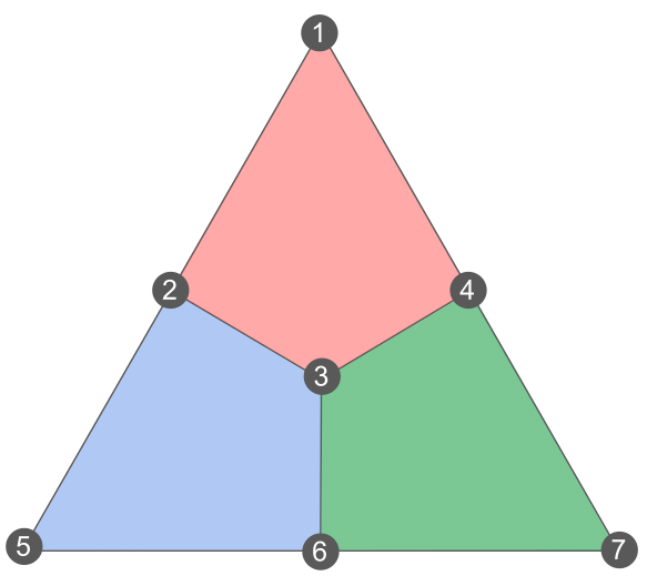
Therefore, the Steane code has six independent stabilizer generators, three \(X\) plaquettes and three \(Z\) plaquettes, such that \(m=6\). Hence we can see that it encodes \(k=7-6=1\) logical qubits.
Pauli logical operators
Now that we know the number of encoded qubits, what about the distance? To describe it, we need to introduce the notion of logical operator. A Pauli logical operator (often abbreviated logical operator, or just logical) is a Pauli operator that commutes with all the stabilizers. In other words, a logical operator is an element of the centralizer \(C(\mathcal{S})\) of the stabilizer group \(\mathcal{S}\), defined as
\[\begin{aligned} C(\mathcal{S})=\{L \in \mathcal{P}_n \,:\, LS = SL,\, \forall S \in \mathcal{S} \} \end{aligned}\]where \(\mathcal{P}_n\) is the \(n\)-qubit Pauli group (all the tensor products of Pauli operators with a phase multiple of \(i\)).
It is easy to show that the set \(\mathcal{L}=C(\mathcal{S})\) of all Pauli logicals from a group, that is, the product of two logicals is itself a logical, and the inverse of a logical is also a logical.
Finally, let’s define non-trivial logical operators (also known as logical errors) as elements of \(\mathcal{C}(\mathcal{S}) \backslash \mathcal{S}\), or in other words, Pauli operators that commute with all the stabilizers but are not stabilizers themselves. We can now characterize the distance of a stabilizer code as the weight of the smallest logical error:
\[\begin{aligned} d = \min_{L \in \mathcal{C}(\mathcal{S}) \backslash \mathcal{S}} |L| \end{aligned}\]As usual, let’s apply what we’ve seen to the Steane code. I claim that the following operators, that we will call \(X_L\) and \(Z_L\), are non-trivial logical operators of the code:
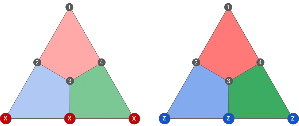
Indeed, it is easy to check that they commute with all the stabilizers, as they share either zero or two qubits with every plaquette. Moreover, by trying all the combinations of stabilizers, you can show that they don’t belong the stabilizer group, and are therefore non-trivial. By using a similar brute-force search, you can also show that they are the smallest non-trivial logical operators, thereby proving that the distance of the Steane code is \(d=3\). This achieves the proof that the Steane code is a \([[7,1,3]]\) code, as claimed in the previous post.
However, we still haven’t shown that \(X_L\) and \(Z_L\) actually act as logical \(X\) and \(Z\) operators on the codespace. For that, we would need to show that \(X_L\) corresponds to a logical bit-flip and \(Z_L\) to a logical phase-flip, i.e. that they map respectively \(\vert 0 \rangle_L\) into \(\vert 1 \rangle_L\) and \(\vert + \rangle_L\) into \(\vert - \rangle_L\). Alternatively, we could show that \(\vert 0 \rangle_L\) and \(\vert 1 \rangle_L\) are eigenstates of \(Z_L\) while \(\vert + \rangle_L\) and \(\vert - \rangle_L\) are eigenstates of \(X_L\).
As it happens, this is just a matter of convention. There is no preferred \(\vert 0 \rangle_L\) state in the codespace, we have the freedom to pick any of the states and decide that it is going to be the zero state. For instance, for the repetition code, we decided that \(\vert 0 \rangle_L=\vert 000 \rangle\), but we could have very much taken \(\vert 0 \rangle_L=\vert 111 \rangle\) or even \(\vert 0 \rangle_L=\frac{1}{\sqrt{2}} \left(\vert 000 \rangle+\vert 111 \rangle\right)\), as long as we keep track of it during the computation and when analyzing the measurements.
Therefore, as it is usually done with stabilizer codes, let’s define \(\vert 0 \rangle_L\) and \(\vert 1 \rangle_L\) as the two eigenstates of \(Z_L\), and \(\vert + \rangle_L\) and \(\vert - \rangle_L\) as the two eigenstates of \(X_L\). This is a valid choice since \(X_L\) and \(Z_L\) anticommute, and this also fixes the logical \(Y\) operator as \(Y_L=iX_LZ_L\).
Logical cosets
In the previous example, we saw one instance of logical \(X\) and \(Z\) operators. However, there will often be multiple logical operators that act as a given Pauli. Indeed, take a logical operator \(L \in \mathcal{L}\) and a stabilizer \(S \in \mathcal{S}\). Then \(SL=LS\) is also a logical operator acting in the same way on the codespace:
\[\begin{aligned} L S \vert \psi \rangle = L \vert \psi \rangle \end{aligned}\]In other words, applying a stabilizer to a logical doesn’t change the way it acts on the codespace. We say that two logicals \(L\) and \(L'\) are equivalent if they only differ by a stabilizer, that is, if there exists \(S \in \mathcal{S}\) such that \(SL=L'\). For instance, we have the following three equivalent logical \(X\) operators in the Steane code:
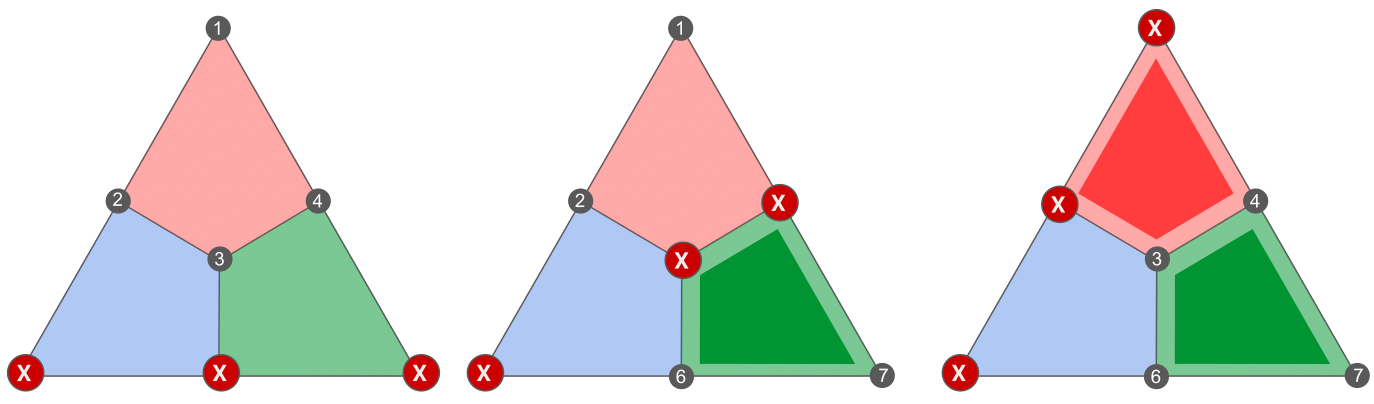
To go from the first one to the second one, we apply a green \(X\) plaquette. To go from the second one to the last one, we apply a red \(X\) plaquette.
Since all the equivalent logicals act in the same way on the codespace, it makes sense to group them together in some ways. The notion of equivalence classes is exactly what we need to formalize this idea.
An equivalence class, or coset, is a set of the form
\[\begin{aligned} \bar{L}=L\mathcal{S}=\{ LS : S \in \mathcal{S} \} \end{aligned}\]where \(L \in \mathcal{L}\) is any logical operator. In other words, a coset is a set of equivalent logicals. Any element \(P \in \bar{L}\) is called a representative of the coset \(\bar{L}\). For instance, any of the three \(X\) logicals of the figure above are representative of the coset \(\bar{X}\) of \(X\) logicals. Note that since the Steane code has only one qubit, all the \(X\) logicals are equivalent and there is only one coset of \(X\) logicals.
Let’s remember a few important properties of equivalence classes. First of all, they partition the set of logical operators, that is, they are all disjoint (i.e. have an empty intersection) and their union is the whole set. In the case of the Steane code, this can be written[^2]:
\[\begin{aligned} \mathcal{L}=\bar{I} \cup \bar{X} \cup \bar{Y} \cup \bar{Z} \end{aligned}\]If we had multiple logical qubits, we would have three different cosets \(\bar{X_i}\), \(\bar{Y_i}\), \(\bar{Z_i}\) for each logical qubit.
Secondly, the set of all the cosets form a group, which is called the quotient group of \(\mathcal{L}\) by \(\mathcal{S}\), and denoted \(\mathcal{L} / \mathcal{S}\). In this group, the multiplication between two cosets \(\bar{L}_1=L_1 \mathcal{S}\) and \(\bar{L}_2=L_2 \mathcal{S}\) is defined as \(L_1 L_2 \mathcal{S}\), where \(L_1\) and \(L_2\) are two arbitrary representatives of \(\bar{L}_1\) and \(\bar{L}_2\). It is a nice exercise to check that the result does not depend on the choice of the two representatives. Moreover, you can check that the identity element of the group is \(\bar{I}=\mathcal{S}\).
Finally, the quotient group can be generated by all the \(\bar{X}_i, \bar{Z}_i\). This means that the number of logical qubits is exactly half the number of generators of \(\mathcal{L}/\mathcal{S}\). This simple fact gives us a different way to count the number of logical qubits of a given stabilizer code, which will become extremely important when discussing topological quantum error correction in future posts.
Conclusion
In this post, we have introduced many crucial concepts to understand stabilizer codes. We have seen that Pauli logical operators correspond to elements of the centralizer, that is, elements that commute with all the stabilizers. We have seen that logical operations are highly degenerate in stabilizer codes, as multiplying a logical operator by a stabilizer gives the same operation on the codespace. We have therefore shown how to group equivalent logicals together within equivalent classes. We have learned how to compute the number of logical qubits in two different ways: either by counting the number \(m\) of generators of \(\mathcal{S}\) and using \(k=n-m\), or by counting the number of generators of \(\mathcal{L} / \mathcal{S}\) and dividing by two. Finally, we have seen that the distance can be obtained by finding the minimum-weight logical operator. All those ideas have been illustrated using the Steane code, which we have proven to be a \([[7,1,3]]\)-code.
In the next and last part of this trilogy, we will see how to formulate the stabilizer formalism in a more concrete way, using parity-check matrices in the binary symplectic format. This format, widely used in numerical implementations of quantum codes, will allow us to switch from group theory to linear algebra. We will express stabilizers and logicals as binary vectors, with commutation relations corresponding to a linear operation on those vectors. Using the notion of logical cosets that we have learned in this post, we will finally be able to formalize the decoding problem for quantum codes.