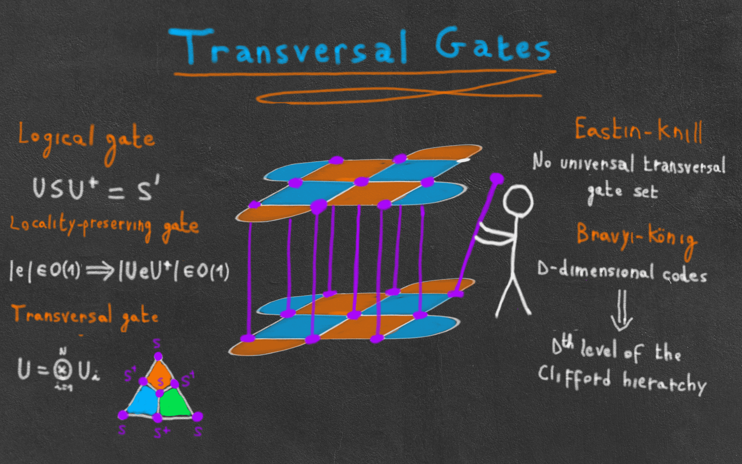
Computing with quantum codes using transversal gates
If you have been following the quantum news lately, you certainly didn’t miss one of the biggest announcements of the year: the demonstration of various quantum codes and logical operations on up to 48 logical qubits and 280 physical qubits of a Rydberg atom array. To me, one of the most exciting features of this experiment is its inherent non-locality: it is possible to apply gates between qubits that are far away by simply moving the corresponding atoms, without inducing more errors than we are able to correct. From a quantum error correction point-of-view, this allows two things: the possibility to create codes beyond two dimensions (such as 3D codes or more general LDPC codes), and the possibility to apply logical two-qubit gates without inducing any additional space-time cost: transversal gates can be used instead of the more common lattice surgery of traditional surface code architectures.
Transversal gates are both the earliest and simplest way to perform computation fault-tolerantly with a quantum code. But those new experimental prospects, along with the recent discovery of many new quantum LDPC codes with great parameters (but not a lot of gates yet!), make research into transversal gates an exciting area again! And if you haven’t had the occasion to learn about them yet, or even logical gates in general, this blog post is for you!
We will start by building up the edifice necessary to understand transversal gates, defining the notions of logical gates, locality-preserving operators and fault-tolerant gates. This will allow us to define transversal gates and understand why they are useful. We will then give a few examples of such gates on both the surface code and the Steane code. Finally, we will study the limitations of transversal gates through the Eastin-Knill and the Bravyi-König theorem, and glimpse at how those limitations can be by-passed when considering non-transversal implementation methods.
Definition and examples
What is a logical gate?
Let’s consider an \([[n,k,d]]\) stabilizer code defined by the stabilizer group \(\mathcal{S}\). A logical unitary gate is a unitary operator \(U\) acting on the \(n\) physical qubits of the code, that preserves its codespace \(\mathcal{C}\), that is
\[\begin{aligned} U \vert \psi \rangle \in \mathcal{C}, \; \forall \vert \psi \rangle \in \mathcal{C} \end{aligned}\]For instance, if we start in a state \(a\vert 000\rangle + b\vert 111\rangle\) in the codespace of the repetition code, we want our logical operation to give us another state \(a'\vert 000\rangle + b'\vert 111\rangle\) within the same codespace. Note that if we take our codespace to be a tensor product of several codespaces, this definition includes multi-qubit logical gates as well (e.g. a \(\texttt{CNOT}\) between two surface codes). Also note that logical gates in general can also include measurements, but for the purpose of this post, we will restrain ourselves to logical unitary gates.
An important observation is that the set of logical unitary gates forms a group: both the product of two logical gates and the inverse of one preserve the codespace. For the inverse, we can see this by writing the unitary as a block diagonal matrix (with two blocks, one acting on the codespace and one acting on the rest of the Hilbert space) and remember that the inverse of a block diagonal matrix consists of the inverse of each block.
Let’s now use the fact that we are dealing with stabilizer codes. By definition of the codespace of a stabilizer code, the definition above can be reformulated as
\[\begin{aligned} S U \vert \psi \rangle = U \vert \psi \rangle, \; \forall S \in \mathcal{S},\; \forall \vert \psi \rangle \in \mathcal{C} \end{aligned}\]Multiplying by \(U^{\dagger}\) on both sides, this is equivalent to:
\[\begin{aligned} U^{\dagger} S U \vert \psi \rangle = \vert \psi \rangle, \; \forall S \in \mathcal{S},\; \forall \vert \psi \rangle \in \mathcal{C} \end{aligned}\]Or, using the fact that the inverse of a logical gate is also a logical gate:
\[\begin{aligned} U S U^{\dagger} \vert \psi \rangle = \vert \psi \rangle, \; \forall S \in \mathcal{S},\; \forall \vert \psi \rangle \in \mathcal{C} \end{aligned}\]In other words, logical gates turn stabilizers into stabilizers! From this point-of-view, it is tempting to redefine logical gates as operators that preserve the stabilizer group. However, this is not exactly true: while elements of the stabilizer group are by definition Pauli operators, there is no constraint for \(USU^\dagger\) to be Pauli. For instance, in the 3D color code, the transversal \(\texttt{T}\) gate turns Pauli \(X\) stabilizers into products of \(S\) gates, which are (non-Pauli) stabilizers, and are therefore outside of \(\mathcal{S}\).
Denoting the group of (both Pauli and non-Pauli) stabilizers by \(\widetilde{\mathcal{S}}\), we can now give the following equivalent definition of a logical gate. A unitary operator \(U\) is a logical gate if and only if
\[\begin{aligned} USU^{\dagger} \in \widetilde{\mathcal{S}}, \; \forall S \in \mathcal{S} \end{aligned}\]So whenever we introduce a new potential logical gate for a given code, the first step is always to verify that it maps Pauli stabilizers to general stabilizers1. The second step is to check what logical operation it performs. Indeed, it is in principle possible that applying Hadamard gates on all the physical qubits ends up implementing a completely different logical gate than a Hadamard. To determine the effect of a logical gate, there are two possibilities:
- We check its effect on logical states. For instance, if we can prove that it maps \(\vert 0\rangle_L\) to \(\vert +\rangle_L\), and \(\vert 1\rangle_L\) to \(\vert -\rangle_L\), it means we are dealing with a logical Hadamard.
- We check its effect on logical Paulis. For instance, showing that \(UX_LU^{\dagger}=Z_L\) and \(UZ_LU^{\dagger}=X_L\) proves that \(U\) is a logical Hadamard (up to a phase). Determining the phase (which is necessary for instance to create a controlled version of the gate) can then be done by checking the effect of U on one chosen logical state.
While we can find examples of the two methods used in the literature, I tend to prefer the second one as the resulting proofs are often easier to visualize.
In this context, it can be useful to memorize how the most important gates transform Pauli operators. Here are a few examples:
- \(\texttt{H}: X \leftrightarrow Z\).
- \(\texttt{S}: X \rightarrow Y\) and \(Z \rightarrow Z\)
- \(\texttt{S}^\dagger: X \rightarrow -Y\) and \(Z \rightarrow Z\)
- \(\texttt{T}: X \rightarrow e^{-i\pi/4} \texttt{SX}\) and \(Z \rightarrow Z\)
- \(\texttt{T}^\dagger: X \rightarrow e^{i\pi/4} \texttt{S}^\dagger\texttt{X}\) and \(Z \rightarrow Z\)
- \(\texttt{CNOT}: XI \rightarrow XX,\; IX \rightarrow IX,\; ZI \rightarrow ZI\) and \(IZ \rightarrow ZZ\) (where the first qubit is the control and the second is the target)
- \(\texttt{CZ}: XI \rightarrow XZ,\; IX \rightarrow ZX,\; ZI \rightarrow ZI\) and \(IZ \rightarrow IZ\)
- \(\texttt{CCZ}: XII \rightarrow X(\texttt{CZ})\) and \(ZII \rightarrow ZII\) (and similarly when putting the \(X\) or \(Z\) on the two other qubits)
What is a fault-tolerant gate?
While our definition of logical gates guarantees that the code itself is preserved, it does not guarantee that the error-correcting properties are. For instance, imagine a code defined on a square grid, with qubits as vertices, and a logical gate made of \(\texttt{CNOT}\)s between disjoint pairs of physical qubits. Something like this:
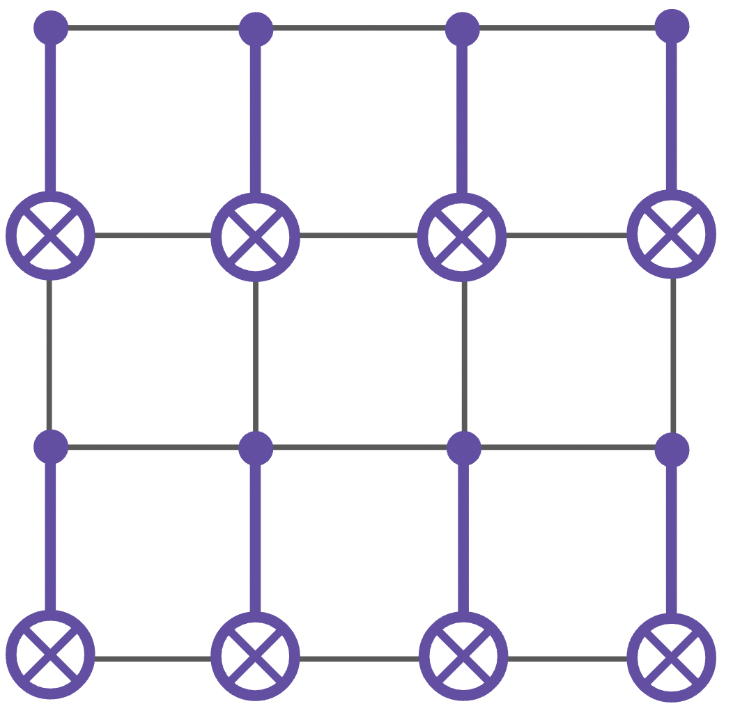
Now, imagine that an \(X\) error appears on the top-left qubit. We can understand how this error propagates by looking at the effect of \(\texttt{CNOT}\) on it. As we saw in the previous section, \(\texttt{CNOT} (XI) \texttt{CNOT}^{\dagger} = XX\), or equivalently \(\texttt{CNOT} (XI) = (XX) \texttt{CNOT}\). This can be visualized by the following circuit:
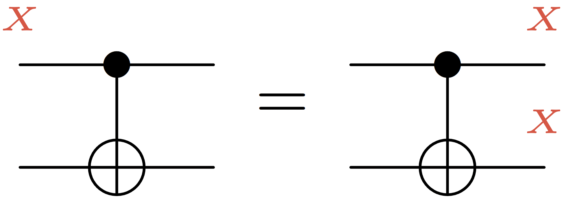
In other words, a single \(X\) error propagates into two \(X\) errors once we have applied our logical gate. Now, let’s suppose that the distance of this code is \(4\) and that any vertical string of \(X\) is an example of minimum-weight logical \(X\) operator. It means that with only \(2\) errors present before applying the gate, we can get a logical error once the gate has been applied. In other words, the effective distance has been reduced by two.
As a second (and even worse!) example, imagine that our \(\texttt{CNOT}s\) were instead acting on intersecting pairs of qubits:
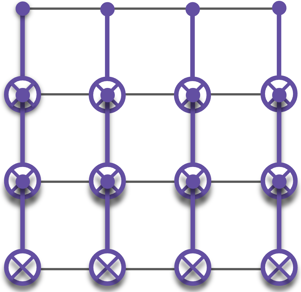
Then, a single qubit \(X\) error can propagate into \(d\) \(X\) errors and create a logical error, effectively reducing the distance to one!
So what is a fault-tolerant logical gate? For a given family of code with a growing distance, a fault-tolerant logical gate is a gate that doesn’t reduce the effective distance (i.e. the minimum number of physical errors that creates a logical error after applying the gate) to \(O(1)\) when the family is growing2. For instance, generalizing the two examples above to families of codes of size \(L \times L\), the first gate would be considered fault-tolerant while the second one wouldn’t.
Within the class of fault-tolerant gates, locality-preserving gates are particularly useful to consider and easier to manipulate in practice. Given a family of codes, a locality-preserving gate is a logical gate \(U\) that transforms small errors to small errors, that is, if \(\bm{e}\) is a Pauli error supported on \(\ell\) qubits, \(UeU^\dagger\) must be supported on \(c \ell\) qubits, where \(c=O(1)\). Again, our first example is locality-preserving while the second one is not. A typical subset of locality-preserving gates is the set of constant-depth quantum circuits.
What is a transversal gate?
Definition
The easiest examples of locality-preserving gates are the transversal gates. To understand them, let’s consider the setting where we are trying to apply a logical gate between multiple copies of a code (e.g. a CNOT between two surface code qubits). Each copy of the code is often called a code block. Transversal gates are logical gates that don’t propagate errors within each code block: one-qubit errors remain one-qubit errors on each code block, thereby preserving the distance. To guarantee this, transversal gates should never couple multiple physical qubits of the same code block. This include logical gates that can be written as a tensor product of single-qubit physical gates only, but also those made of multi-qubit gates connecting qubits of different code blocks.
For instance, Pauli gates are transversal for all stabilizer codes, since by definition Pauli logicals can always be written as a tensor product of Pauli operators. But, as we will soon see, the gate made of \(\texttt{CNOT}\)s between corresponding qubits on two code blocks also implements a transversal \(\texttt{CNOT}\) for any CSS code:
![]()
Example 1: Steane code
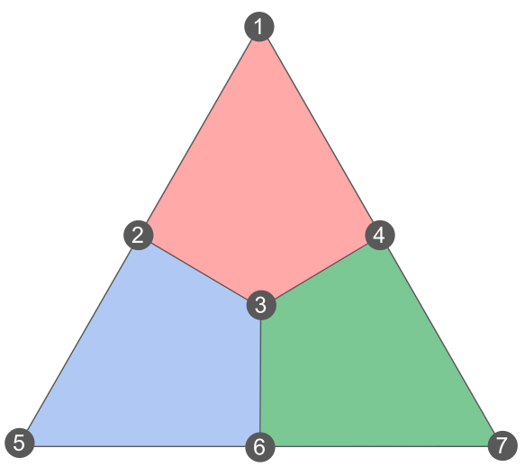
Let’s take a look at some examples of transversal gates in codes that we know. Let’s start with the Steane code. As a reminder, the Steane code is defined on the following lattice, where qubits are on vertices, and \(X\) and \(Z\) stabilizers on faces:
Let’s consider the gate made of \(\texttt{H}\) acting on every qubits. Is it a logical gate? To determine this, let’s see how it transforms stabilizers. Since \(\texttt{H}\) transforms \(X\) into \(Z\), and vice-versa, it means that any plaquette stabilizer \(XXXX\) will turn into \(ZZZZ\) supported on the same plaquette, and similarly, any stabilizer \(ZZZZ\) will turn into \(XXXX\). Since the resulting operators are stabilizers as well, it means that our gate preserves the stabilizer group! So it’s a logical gate.
What is the effect of this logical gate? Let’s see how it transforms the logical Paulis. For that, we can pick any representative Pauli \(X\) and \(Z\) logical, such as those:
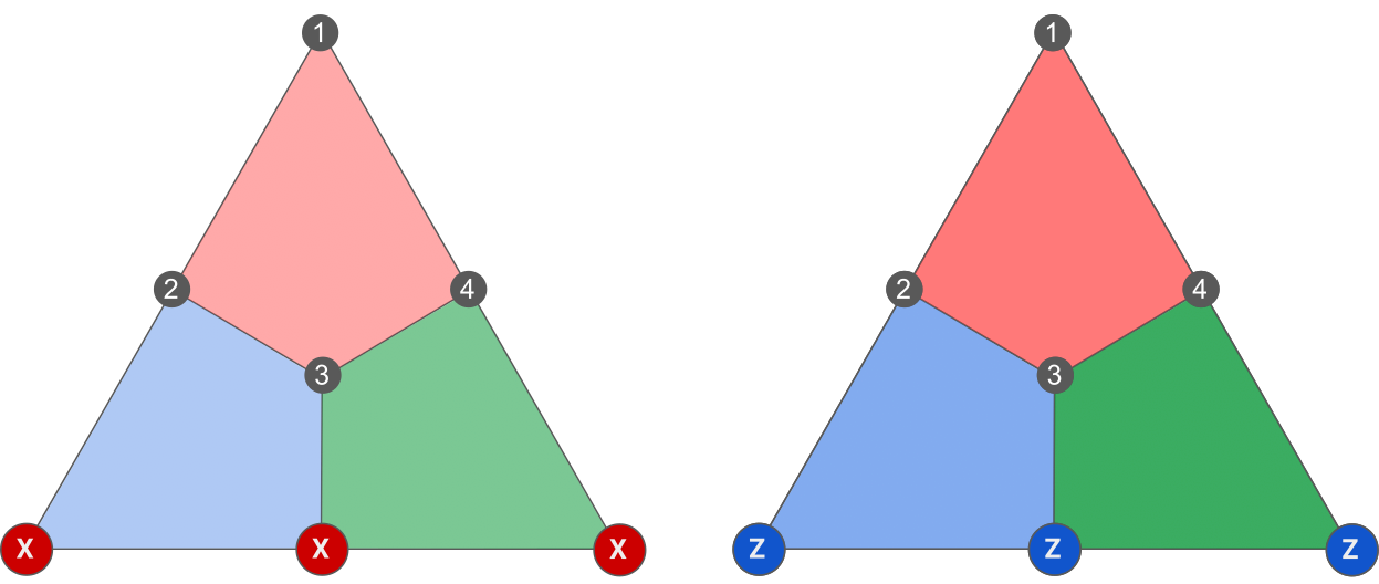
Since our gate turns \(XXX\) into \(ZZZ\) and vice-versa, it means that it exchanges \(X_L\) and \(Z_L\) and is therefore a logical Hadamard up to a phase. The following exercise shows that this phase is actually \(1\).
Can we also implement an \(\texttt{S}\) gate transversally? Let’s see what happens when we apply \(\texttt{S}\) to all the physical qubits. Since \(\texttt{S}X\texttt{S}^\dagger=Y\), every \(X\) plaquette will turn into \(Y^{\otimes 4}\) under the action of our gate. Now, is \(Y^{\otimes 4}\) a stabilizer? Since \(Y^{\otimes 4}=(iXZ)^{\otimes 4}=X^{\otimes 4} Z^{\otimes 4}\), with both \(X^{\otimes 4}\) and \(Z^{\otimes 4}\) being stabilizers supported on the same plaquette, we see that \(Y^{\otimes 4}\) is indeed a stabilizer. Moreover, since \(\texttt{S}Z\texttt{S}^\dagger=Z\), \(Z\) plaquettes are preserved. Hence, our gate preserves the codespace and is therefore a valid transversal logical gate!
Let’s now look at the action of our gate on the logicals. For our gate to be a logical \(\texttt{S}\) gate, we would need to prove that \(\texttt{S} \bar{X} \texttt{S}^\dagger = \bar{Y}\). Picking the logical \(X\) representative supported on three qubits from the figure above, we can see that the gate turns \(\bar{X}\) into \(Y^{\otimes 3}\). But \(Y^{\otimes 3}=(iXZ)^{\otimes 3}=-iX^{\otimes} Z^{\otimes 3}=-i\bar{X} \bar{Z}=-\bar{Y}\). So \(\texttt{S}^{\otimes 7}\) turns any \(X\) logical into a \(-Y\) logical. Thus, perhaps surprisingly, what our gate actually implements is a logical \(\texttt{S}^\dagger\)!
To implement an actual logical \(\texttt{S}\), one simple solution is to instead apply \(\texttt{S}^\dagger\) everywhere. But there exists many more solutions. For instance, a solution that generalizes well to color codes (which we will see in a future post), is to take a bipartition of the qubits of the Steane code, that is, divide the vertices into two colors (black and white), such that two vertices of the same color are never incident to each other through an edge:
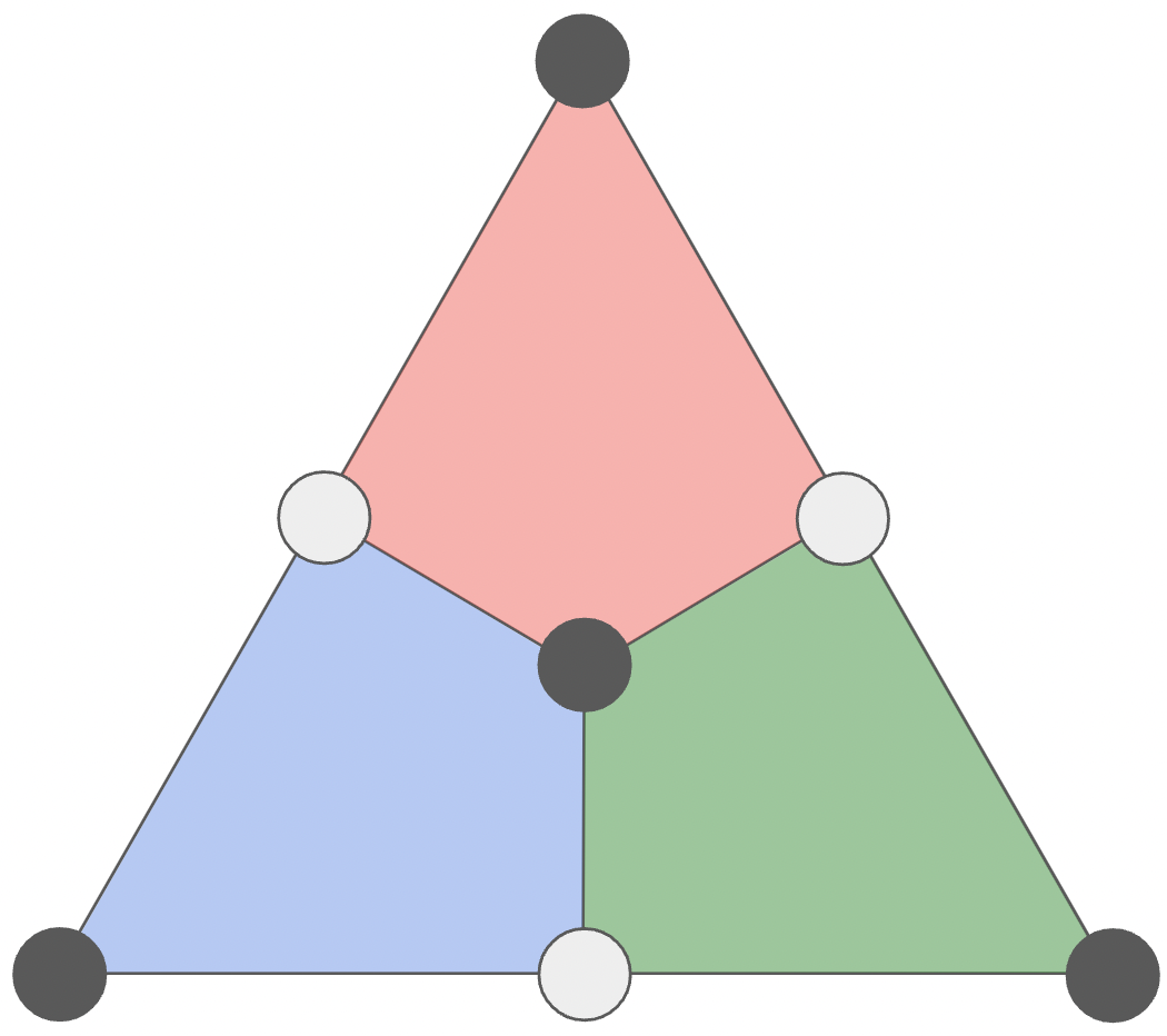
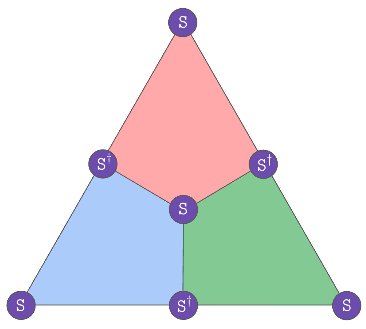
Since we have an odd number of qubits, one color will contain more vertices than the other. In the drawing above, there are more black vertices than white vertices. However, every plaquette contains the same number of white and black qubits. Now, let’s apply \(\texttt{S}\) to the four black qubits, and \(\texttt{S}^\dagger\) to the three white qubits. Using the same calculation techniques as above, it should be an easy exercise to show that this gate also implements a logical \(\texttt{S}\):
Since we are on a good streak, let’s go on and look at the \(\texttt{T}\) gate! Can we implement a \(\texttt{T}\) gate transversally on the Steane code? Unfortunately, the answer is no this time. For instance, try to show that using a combination of \(\texttt{T}\) and \(\texttt{T}^\dagger\) on all qubits does not implement a logical gate at all:
More generally, we will soon see that it is not possible to implement non-Clifford gates transversally on 2D codes, so this eliminates any other possibility of transversal \(\texttt{T}\) gate on the Steane code.
There’s one last important gate that we can implement transversally on the Steane code: the \(\texttt{CNOT}\) gate. As a matter of fact, \(\texttt{CNOT}\) is transversal for any CSS code! Indeed, \(\texttt{CNOT}\) maps \(X \otimes I\) to \(X \otimes X\), \(I \otimes Z\) to \(Z \otimes Z\), and preserves \(I \otimes X\) and \(Z \otimes I\). So any \(X\) stabilizer \(S_X\) of the control code will be mapped to \(S_X \otimes S_X\), which stabilizes the tensor product of the two codes, and similarly for \(Z\) stabilizers on the target code. So the transversal \(\texttt{CNOT}\) gate preserves the stabilizer group and is therefore a valid logical gate. Moreover, it will map any logical \(X\) representative of the control code to a logical \(X \otimes X\) representative of the two codes, and similarly for the \(Z\) logicals of the target code, thereby implementing a logical \(\texttt{CNOT}\).
However, despite its simplicity, the transversal \(\texttt{CNOT}\) is often too impractical when dealing with a planar architecture. Indeed, to implement it physically, it requires either putting one code block above the other or having long-range connections. Alternatively, methods based on lattice surgery or code deformation, that I will discuss in a separate blog post, only use geometrically-local operations in 2D, making it more practical on planar architectures. On architectures that are not restricted to 2D operations, such as the one I was talking about in the intro, the transversal \(\texttt{CNOT}\) is however perfectly valid and has even been implemented in real life!
Example 2: Surface code
The biggest advantage of the Steane code (and more generally, color codes) is the ease with which it can implement the full Clifford group transversally. As we will now see, things gets a bit trickier with surface codes.
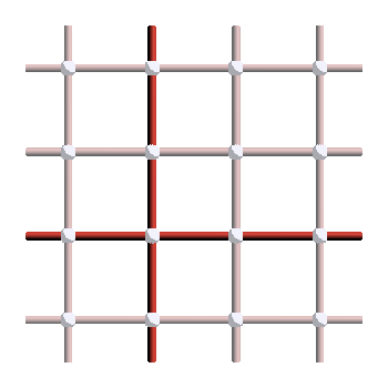
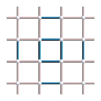
Let’s start by considering an non-rotated surface code with periodic boundary conditions. We put qubits on edges, \(X\) stabilizers (red) on plaquettes and \(Z\) stabilizers (blue) on vertices:
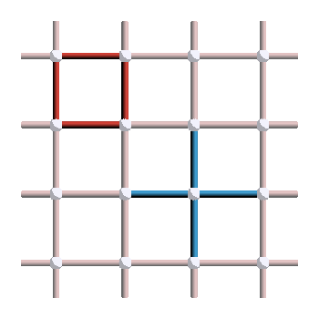
As a reminder, this version of the surface code encodes two logical qubits, whose logical \(X\) and \(Z\) operators correspond to the two types of non-trivial loops of the torus, in the primal and dual pictures respectively:
So what happens when we apply a Hadamard gate on all physical qubits of the code? It turns the \(X\) plaquette stabilizers into \(Z\) plaquette operators, and the \(Z\) vertex stabilizers into \(X\) vertex operators. Since \(Z\) plaquette and \(X\) vertex operators are not stabilizers of the surface code we are considering, the operation is not a logical gate according to our definition. However, that’s where we might want to loosen our definition a little: the code resulting from the application of \(\texttt{H}\) everywhere is still a valid surface code, with just a different convention for which stabilizers are \(X\) or \(Z\). Since we have periodic boundary conditions, this code transformation can also be seen as a simple translation by half an edge in the horizontal and vertical directions. Moreover, \(X\) logicals of the initial code are turned into \(Z\) logicals of the new code, so the operation corresponds to a logical Hadamard applied simultaneously to the two logical qubits of the toric code. So, as long as we keep track of what the stabilizers are at every instant, we are in principle allowed to modify the code when applying logical gates (particularly if the new code is just a translation or rotation of the original one).
More care is needed when considering this operation on the planar code, in the context of a broader quantum circuit. Indeed, when using a rotated planar code, we can see the code resulting from the application of the transversal Hadamard as a rotation of the original code.
Now, let’s imagine that we would like to apply a \(\texttt{CNOT}\) after the Hadamard. In most proposed fault-tolerant architectures based on the surface code, \(\texttt{CNOT}\)s are done using code deformation or lattice surgery. And for those to work, we need \(X\) and \(Z\) logicals to be aligned on all the different patches of surface code. So to recover the original code with logicals aligned as before, we need to somehow rotate the code back. This can be done either by physically moving the qubits around, which is often not feasible in the context of a 2D architecture, or by applying some operations to perform the rotation without moving qubits. This can be done fault-tolerantly using lattice surgery on some ancilla patches, and a few \(\texttt{SWAP}\) gates. In summary, it is possible to implement the Hadamard gate transversally on the surface code, but on a planar architecture, this requires some lattice surgery if we want to apply logical gates afterwards.
What about the \(\texttt{S}\) gate? Applying it on all physical qubits turns \(X\) stabilizers into \(Y\) stabilizers, and preserves the \(Z\) ones. This “ZY surface code” defines a valid code, and you can check that the transversal \(\texttt{S}\) has the right effect on the logicals. However, contrary to the Hadamard case, this new code is not a simple translation or rotation of the original surface code, it is a fundamentally different code with a different set of transversal gates. For instance, it is lacking a transversal \(\texttt{CNOT}\) (as a non-CSS code), which is replaced by a transversal \(\texttt{S} \; \texttt{CNOT} \; \texttt{S}^\dagger\). But applying this newly-available gate after having applied a transversal \(\texttt{S}\) gate would undo the \(\texttt{S}\), defeating the purpose of having it. I believe that a similar reasoning could be done when considering \(\texttt{CNOT}\)s implemented through lattice surgery. More generally, to design a complete architecture with a universal set of gates, imposing that gates preserve the codespace (potentially up to an isomorphism of the Tanner graph, like a rotation or translation of the code) is required. We therefore conclude that, contrary to the Steane code, the \(\texttt{S}\) gate is not available transversally on the surface code. As we will see in different posts, there are other ways to implement it, such as state injection, braiding, or fold-transversality.
What about other gates? Similarly to the Steane code, non-Clifford gates such as \(\texttt{T}\) are not available on the surface code. Let’s now try to understand why using more general results in the field.
Limitations on transversal gates
Now that we have understood how transversal gates work, let’s take a step back and try to answer the following question: given any stabilizer code, what types of gate can be implemented transversally? As we will see in this section, the answer is a resounding not enough. The Eastin-Knill theorem states that no universal gate set can be fully implemented transversally, while the Bravyi-König theorem states that the subset of gates that can be implemented transversally depends on the dimension of the code.
Eastin-Knill theorem
Let’s start with the Eastin-Knill theorem. The statement of the theorem from the original paper is the following:
Let’s try to understand what that means. First, the theorem imposes a limit on logical unitary product operators. For any partition of our physical qubits into \(m\) subsystems \(\{ \mathcal{Q}_i \}_{1 \leq i \leq m}\), each of dimension \(d_i\), a logical unitary product operator is a logical operator of the form \(\otimes_{i=1}^m U_i\) where each \(U_i\) acts on subsystem \(\mathcal{Q}_i\). For instance, if we pick each \(\mathcal{Q}_i\) to contain exactly one physical qubit, those are exactly transversal operators.
Then, any local-error-detecting quantum code is concerned by this theorem. The notion of locality here is induced by the partition of our physical qubits. More precisely, a local error here is an error supported on a given subsystem, and the only assumption of our code is that those errors can be detected. This is translated mathematically by the so-called Knill-Laflamme condition, stating that \(P E P \propto P\) for all local errors, where \(P\) is the projector into the codespace. For instance, restricting ourselves to transversal gates, any stabilizer code with a distance \(d \geq 2\) will be concerned by this theorem.
Finally, what is a universal gate set? It is a gate set that can approximate any unitary in \(U(2^n)\) up to arbitrary precision. For instance, the set generated by the gates \(\{ \texttt{H}, \texttt{CNOT}, \texttt{T} \}\), i.e. that contains all the products of those gates, is universal.
How is the Eastin-Knill theorem proven? The main idea is to show that the group of logical unitary product operators is finite, while any universal gate set is infinite. The technical details of the proof rely on the theory of Lie groups and algebras, and would require a separate post (in preparation!) to discuss properly.
While the application domain of this theorem is already quite large—it applies both beyond stabilizer codes and beyond transversal gates—it has been generalized even further in the literature. For instance, the same limit applies when looking at locality-preserving gates in general, rather than product operators.
Bravyi-König theorem
The Bravyi-König theorem states that the transversal gates (or more generally the gates implemented by a constant-depth quantum circuit) of a \(D\)-dimensional quantum code are limited to the \(D\)-th level of the Clifford hierarchy. The \(n\)-qubit Clifford hierarchy \(\left(\mathcal{P}_j\right)_{j \geq 1}\) is a family of sets of unitaries that can be defined by induction as follows:
- The first element \(\mathcal{P}_1\) is the \(n\)-qubit Pauli group.
- The \(j\)-th element \(\mathcal{P}_j\) is the set of \(n\)-qubit unitaries \(U\) such that \(U \mathcal{P}_1 U^{\dagger} \subseteq \mathcal{P}_{j-1}\).
For instance, \(\mathcal{P}_2\) is the set of all unitaries such that \(U \mathcal{P}_1 U^{\dagger} \subseteq \mathcal{P}_{1}\), or in other words, all the unitaries that preserve the Pauli group. This is known as the Clifford group, which can be generated by \(\{\texttt{H}, \texttt{S}, \texttt{CNOT}\}\). An important characteristic of the Clifford group is that it is not universal, and any circuit starting from the \(\vert 0 \rangle\) state and consisting uniquely of Clifford gates can be simulated efficiently on a classical computer (using the stabilizer tableau formalism). Universality is achieved from the next element of the Clifford hierarchy, \(\mathcal{P}_3\), which contains gates such as \(\texttt{T}\) and \(\texttt{CCX}\). More generally, \(\mathcal{P}_j\) contains \(\texttt{R}_k=\begin{pmatrix} 1 & 0 \\ 0 & e^{2i\pi/2^{j}} \end{pmatrix}\) and \(\texttt{C}^{j-1} \texttt{X}\).
Let’s now state the theorem as originally formulated in the Bravyi-König paper:
Applying this theorem to 2D codes, we see that they have their transversal gates limited to the Clifford group, so no hope of finding a transversal \(T\) gate on the 2D surface or color code. This justifies the need for magic-state distillation, a method to implement a \(T\) gate (or any other non-Clifford gate) using state injection (more on that in the next section).
What about 3D codes? Those can in principle implement transversal non-Clifford gates, which is one of their key advantages. For instance, the 3D toric code has a transversal CCZ, and the 3D color code (with open boundaries) has a transversal T. However, you might object, doesn’t the Eastin-Knill theorem also apply to 3D codes, meaning that their transversal gate set is still not universal? That’s right! For example, the 3D toric code doesn’t have a transversal Hadamard gate. But as we will discuss in the next section, the key difference with the 2D case is that it is much less costly to implement a fault-tolerant \(\texttt{H}\) than a fault-tolerant \(\texttt{T}\) non-transversally using state injection.
Note that the Bravyi-König theorem can also be generalized to subsystem codes.
How can we circumvent those limitations?
While those two theorems put severe restrictions on how to implement fault-tolerant gates on quantum codes, there are many ways to circumvent them! The general idea is that those theorems apply to unitary implementations only. So implementations involving measurements do not fall under the assumptions of Eastin-Knill and Bravyi-König!
One example of non-transversal method to implement a logical gate is through state injection, where a certain ancilla state is coupled to our qubit, and a conditional measurement is used to implement a gate on this qubit. For instance, an \(\texttt{H}\) gate can be implemented by preparing an ancilla qubit in the \(\vert+\rangle\) state and using the following circuit:
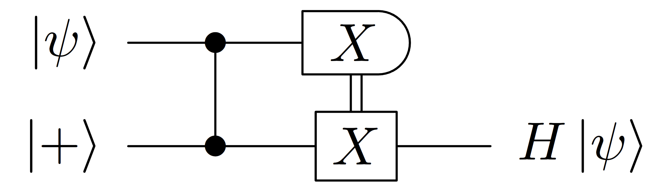
So for a given code, if there exists a method to prepare it in the logical \(\vert+\rangle_L\) state (which is often the case, just exchange \(X\) and \(Z\) stabilizers when preparing the state) and to implement a logical \(\texttt{CZ}\) gate, then it’s possible to implement the Hadamard gate as well. It is for instance the case of the 3D toric code, which has a transversal \(\texttt{CZ}\) and \(\texttt{CCZ}\) but no transversal \(\texttt{H}\). Using Hadamard state injection allows to get a universal logical gate set on this code. So why isn’t everyone using 3D toric codes to perform encoded computation? Apart from the experimental challenges, I would say that the main reason is the lack of evidence that this method, when considered in an end-to-end architecture, actually reduces the overhead compared to more traditional techniques (we even have evidence of the opposite). This is mainly due to 3D codes having a worse distance scaling than 2D codes.
A more common example of state injection is magic state distillation, where an approximation of the state \(\texttt{T} \vert + \rangle_L\) (a so-called magic state) is prepared and injected onto a code using the following circuit
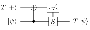
This results in a \(\texttt{T}\) gate being applied to the code. The main difficulty of this method comes from the preparation of the magic state, and countless papers and theses have been written on this topic! The main idea is to start with a noisy \(T\) state and distill it into a clean one, often using quantum codes that can implement \(\texttt{T}\) gates transversally in the process. Magic state distillation is for instance the preferred method to implement the \(\texttt{T}\) gate on the surface code.
Another method to implement logical gates fault-tolerantly is code switching, where measurements are used to switch between two codes with different sets of transversal gates, while preserving the logical information. For instance, code switching between the 2D and 3D color code allows to implement both the \(\texttt{T}\) gate (using the 3D color code) and the \(\texttt{H}\) gate (using the 2D color code), which make up a universal gate set when adding \(\texttt{CNOT}\) (implementable on both codes).
Conclusion
In this post, we looked at the definition of logical gates—operations that preserve the codespace—, fault-tolerant gates—operations that don’t propagate errors uncontrollably—, and transversal gates—operations that don’t propagate errors at all within a codeblock. After studying proof techniques to show that a gate is a logical gate, we considered a few examples of transversal gates in codes that you know. In particular, we showed that the Steane code can implement the full Clifford group transversally, while the surface code only has the Hadamard gate available (modulo a rotation of the code). Finally, we looked at general limitations on transversal gates through the Eastin-Knill and the Bravyi-König theorem. Due to those limitations, we discussed how many other methods are available to circumvent those theorems and implement logical gates fault-tolerantly. Therefore, there is much more to say about logical gates and I hope to continue this series with topics such as lattice surgery, fold-transversality, braiding, code switching, etc.
However, despite this abundance of more complicated techniques to implement logical gates, research in transversal gates is still very much active and many open questions remain to be answered. In particular, with the recent rise of new qubit architectures which are not constrained by locality and of new LDPC codes which exploit this non-locality to drastically improve the (asymptotic) qubit overhead of quantum codes, transversal gates are becoming popular again. For instance, implementing a CNOT transversally by moving qubits that are far away close to each other could be less costly than performing lattice surgery (which involves the use some ancilla patches). But all the transversal gates of those LDPC codes have very much not been figured out. Only recently have the first codes with a constant rate and some transversal non-Clifford gates been found. Finding non-Clifford transversal gates on good LDPC codes (i.e. with a constant rate AND a linear distance) with extensive addressability (i.e. where logical gates could be implemented on all logical qubits, or pairs of logical qubits, individually) could result in very low-overhead fault-tolerant architectures.
Solution of the exercise
-
In practice, if \(U^{\dagger}SU\) is not a Pauli, it is often more involved to show that it’s a stabilizer. The most general method, that you find in many papers, is to explicitly write the states of the codespace and show that it stabilizes them. However, my favorite method is to show that \(U^{\dagger}SU\) is itself a logical gate, acting as the identity (i.e. mapping \(X_L\) to \(X_L\) and \(Z_L\) to \(Z_L\)). To show that \(U^{\dagger}SU\) is a logical gate, you either show that it maps Pauli stabilizers to Pauli stabilizers (which is the case in all the situations I’ve encountered), or you recursively continue this process until the operator maps Pauli stabilizers to Pauli stabilizers. We will revise this and look at some explicit examples when talking about 3D codes in a future post, so don’t dwell on that if you find this method a bit abstract at the moment. All our examples of logical gate in this post will map Paulis to Paulis. ↩︎
-
We can find many definitions (as well as absence of definitions) of fault-tolerance in the literature. One of the most formal and general ones is due to Gottesman and can be found here (Sec. 4.2). However, in practice, not reducing the distance to a constant seems to be a good effective definition that is implied in many papers. Alternatively, depending on the context, it could also be useful to impose no more than a constant multiplicative reduction of the distance, or even no reduction at all (for instance if we want to talk about the fault-tolerance of a gate on a specific small code instead of a whole family). But I hope you get the idea. ↩︎