The stabilizer trilogy III — Parity-check matrices and decoding

28 Mar 2023 on Quantum Computing

Welcome to the third and last post of the stabilizer trilogy! In Parts I and II, we introduced the stabilizer formalism using a group theoretic language: stabilizer codes are abelian subgroups of the Pauli group, logicals are elements of the centralizers, etc. While this formulation has a lot of merit, it might not be immediately obvious how to implement it in practice if you want to simulate a code. Fortunately, the whole formalism can be reexpressed using vectors, matrices and the whole linear algebra toolbox that comes with them: this is the parity-check matrix formulation! Parity-check matrices make it not only easy to implement stabilizer codes in your favorite programming language, they are also a very powerful tools to prove theorems about them, to classify them, to decode them, and more!

In this post, we will see how to define the parity-check matrix of a stabilizer code in the binary symplectic format, and how to express the decoding problem using it. After a short motivation section to remind you about classical parity-check matrices, we will delve into the binary symplectic format, a way to express Pauli operators using vectors. We will then define quantum parity-check matrices in this format and see how syndromes and logical operators can be expressed using them. With those tools in our hand, we will finally be able to define the decoding problem for quantum codes, and in particular see how to decode the Steane code. We will finish this post by defining quantum Tanner graphs, a graphical representation of parity-check matrices, often used in the literature to study the properties of codes and decoders.

Motivation

When studying classical coding theory, we saw that a code can be defined as a binary matrix $\bm{H}$, called the parity-check matrix, such that any codeword $\bm{x}$ satisfies

$$\begin{aligned} \bm{H} \bm{x} = \bm{0} \end{aligned}$$

Thus, a codeword $x$ corrupted by an error $\bm{e}$, denoted $\widetilde{\bm{x}}=\bm{x} + \bm{e}$, obeys

$$\begin{aligned} \bm{H} \widetilde{\bm{x}} = \bm{H} \bm{e} = \bm{s} \end{aligned}$$

where $\bm{s}$ is the syndrome. This formulation of linear coding theory was useful for many reasons:

• It allows to express the decoding problem as a constrained optimization problem

$$\begin{aligned} \max_{\bm{e} \in \mathbb{Z}_2^n} P(\bm{e}) \; \text{ s.t. } \; \bm{H} \bm{e} = \bm{s} \end{aligned}$$

• It makes syndrome calculations straightforward, as a simple matrix multiplication
• Many properties of a code can be deduced directly from its parity-check (such as the weight of its checks via the sparsity of the matrix, the number of encoded qubits via its rank, etc.)
• The parity-check matrix can be seen as the adjacency matrix of a graph, the Tanner graph, which is used for instance when solving the decoding problem with belief propagation.

We will now see that such a formulation is possible in the stabilizer formalism. There are two different methods to arrive at a definition of a quantum parity-check matrix:

1. The $GF(4)$ format, where the elements of the parity-check matrix belong to a Galois field with four elements (instead of the binary field in the classical case).
2. The binary symplectic format, where the parity-check matrix remains binary, but doubles in size compared to the classical one.

Even though the $GF(4)$ format has some useful applications¹, the binary symplectic one is simpler, more popular, and used in most quantum error correction libraries². This is therefore the one I will present in this post. Until I do a separate post on $GF(4)$, feel free to take a look at Section 3.2 of Daniel Gottesman’s lecture notes in the meantime.

Binary symplectic format

The core idea behind the binary symplectic format is the observation that Paulis can be mapped to two-bit words using the following dictionary:

$$\begin{aligned} (0\vert0) & \rightarrow I \\ (1\vert0) & \rightarrow X \\ (0\vert1) & \rightarrow Z \\ (1\vert1) & \rightarrow Y \end{aligned}$$

In this representation, the first bit indicates the presence of an $X$ and the second bit the presence of a $Z$. So $(0\vert0)$ is the identity operator (no $X$, no $Z$) and $(1\vert1)$ is the $Y$ operator (as it can be written $XZ$). We can also write this more formally as $(x \vert z) \leftrightarrow X^{x} Z^{z}$.

Since Pauli elements can also have a phase (which can be $+1$, $-1$, $+i$ or $-i$), we should in principle include two more bits in our dictionary in order to represent it. While some applications do require those two bits, e.g. the stabilizer tableau method for simulating Clifford circuits efficiently, the phase is often ignored in the context of quantum error correction. To understand why, let’s consider a quantum code characterized by a stabilizer group $\mathcal{S}$ generated by some elements $\{S_i\}$. Since Pauli elements with a phase of $+i$ or $-i$ are not Hermitian (and furthermore, square to $-I$), they cannot be included in the stabilizer group. Moreover, any time a stabilizer $S_i$ has a phase of $-1$, it’s possible to replace it by $-S_i$ without changing any property of the code. So choosing to have stabilizer generators with a phase of $+1$ or $-1$ is a matter of convention, and the choice of $+1$ for every generator is often adopted. Furthermore, Pauli errors can also be considered to have a phase of $+1$ (in that case, the phase is global and can safely be ignored), and all the important operations considered in this post (such as commutation and anticommutation of Paulis) are phase-independent as well.

One nice feature of our binary representation is that the multiplication of Pauli elements maps to the addition (modulo 2) of two-bit words ³. Indeed,

$$\begin{aligned} (x \vert z) + (x' \vert z') = (x+x' \vert z+z') \leftrightarrow \left( X^{x} Z^{z} \right) \left( X^{x'} Z^{z'} \right) = X^{x+x'} Z^{z+z'} \end{aligned}$$

We were able to commute things through in the last equality as Pauli operators commute up to a phase, which we’re choosing to ignore here.

For instance, $(1\vert0) + (0\vert1) = (1\vert1) \leftrightarrow XZ = Y$, or $(1\vert0) + (1\vert0) = (0\vert0) \leftrightarrow X^2 = I$.

This representation can be generalized to many-qubit Pauli operators as well. A Pauli vector $P=P_1 \otimes \ldots \otimes P_n$ is mapped to the following vector in the binary symplectic format:

$$\begin{aligned} (x_1 \ldots x_n \vert z_1 \ldots z_n) \end{aligned}$$

where $(x_i \vert z_i)$ is the representation of $P_i$. For example, the operator $Z \otimes Y$ can be written $(01 \vert 11)$.

The next step is to express commutation relations in this format. Indeed, remember that the syndrome depends entirely on the commutation relations between stabilizers and errors (the syndrome is $0$ if they commute and $1$ if they anticommute). This is where the “symplectic” part of the binary symplectic format kicks in.

Let’s define the symplectic product $\odot$ between two binary symplectic vectors $(\bm{x} \vert \bm{z})$ and $(\bm{x'} \vert \bm{z'})$ as

$$\begin{aligned} (\bm{x} \vert \bm{z}) \odot (\bm{x'} \vert \bm{z'}) = (\bm{x} \vert \bm{z}) \Omega (\bm{x'} \vert \bm{z'})^T = \bm{x} \cdot \bm{z'} + \bm{z} \cdot \bm{x'} \end{aligned}$$

where $\Omega$ is the symplectic matrix, defined as:

$$\begin{aligned} \Omega = \left( \begin{matrix} 0 & I_n \\ I_n & 0 \end{matrix} \right) \end{aligned}$$

and $\cdot$ is the usual dot product modulo $2$. The interpretation of this product is that two Pauli operators commute if their binary symplectic product is $0$, and anticommute if it is $1$. To see this, notice that $x_i z'_i + z_i x'_i$ is equal to $1$ if and only if there is an $X$ and a $Z$ intersecting on qubit $i$, but not a $Y$ on both (which would give $2$, or $0$ modulo $2$). In other words, it is $1$ if and only if the two Pauli elements acting on qubit $i$ anticommute. Summing over all $i$, it means that the symplectic product $\bm{x} \cdot \bm{z'} + \bm{z} \cdot \bm{x'}$ is equal to $1$ if and only if there is an odd number of Pauli elements that anticommute, or equivalently, if the two Pauli operators anticommute.

The quantum parity-check matrix

We are now ready to talk about parity-check matrices. Let $\mathcal{S}$ a stabilizer group on $n$ qubits, generated by a set of $m$ stabilizers $\{S_i\}$. The quantum parity-check matrix of the code, associated to those generators, is the $m \times 2n$ matrix where each row is a stabilizer written in the binary symplectic format. For example, here is the parity-check matrix of the Steane code, with the plaquette stabilizers as generators:

$$\begin{aligned} \bm{H} = \left( \begin{matrix} \color{OrangeRed} 1 & \color{OrangeRed} 1 & \color{OrangeRed} 1 & \color{OrangeRed} 1 & \color{OrangeRed} 0 & \color{OrangeRed} 0 & \color{OrangeRed} 0 & \vert & \color{OrangeRed} 0 & \color{OrangeRed} 0 & \color{OrangeRed} 0 & \color{OrangeRed} 0 & \color{OrangeRed} 0 & \color{OrangeRed} 0 & \color{OrangeRed} 0 \\ \color{RoyalBlue} 0 & \color{RoyalBlue} 1 & \color{RoyalBlue} 1 & \color{RoyalBlue} 0 & \color{RoyalBlue} 1 & \color{RoyalBlue} 1 & \color{RoyalBlue} 0 & \vert & \color{RoyalBlue} 0 & \color{RoyalBlue} 0 & \color{RoyalBlue} 0 & \color{RoyalBlue} 0 & \color{RoyalBlue} 0 & \color{RoyalBlue} 0 & \color{RoyalBlue} 0 \\ \color{ForestGreen} 0 & \color{ForestGreen} 0 & \color{ForestGreen} 1 & \color{ForestGreen} 1 & \color{ForestGreen} 0 & \color{ForestGreen} 1 & \color{ForestGreen} 1 & \vert & \color{ForestGreen} 0 & \color{ForestGreen} 0 & \color{ForestGreen} 0 & \color{ForestGreen} 0 & \color{ForestGreen} 0 & \color{ForestGreen} 0 & \color{ForestGreen} 0 \\ \color{OrangeRed} 0 & \color{OrangeRed} 0 & \color{OrangeRed} 0 & \color{OrangeRed} 0 & \color{OrangeRed} 0 & \color{OrangeRed} 0 & \color{OrangeRed} 0 & \vert & \color{OrangeRed} 1 & \color{OrangeRed} 1 & \color{OrangeRed} 1 & \color{OrangeRed} 1 & \color{OrangeRed} 0 & \color{OrangeRed} 0 & \color{OrangeRed} 0 \\ \color{RoyalBlue} 0 & \color{RoyalBlue} 0 & \color{RoyalBlue} 0 & \color{RoyalBlue} 0 & \color{RoyalBlue} 0 & \color{RoyalBlue} 0 & \color{RoyalBlue} 0 & \vert & \color{RoyalBlue} 0 & \color{RoyalBlue} 1 & \color{RoyalBlue} 1 & \color{RoyalBlue} 0 & \color{RoyalBlue} 1 & \color{RoyalBlue} 1 & \color{RoyalBlue} 0 \\ \color{ForestGreen} 0 & \color{ForestGreen} 0 & \color{ForestGreen} 0 & \color{ForestGreen} 0 & \color{ForestGreen} 0 & \color{ForestGreen} 0 & \color{ForestGreen} 0 & \vert & \color{ForestGreen} 0 & \color{ForestGreen} 0 & \color{ForestGreen} 1 & \color{ForestGreen} 1 & \color{ForestGreen} 0 & \color{ForestGreen} 1 & \color{ForestGreen} 1 \\ \end{matrix} \right) \end{aligned}$$

I have colored each row in accordance to the plaquette it corresponds to. For convenience, here are the plaquette stabilizers of the Steane code again:

Exercise: Write the parity-check matrix of Shor’s code (solution)

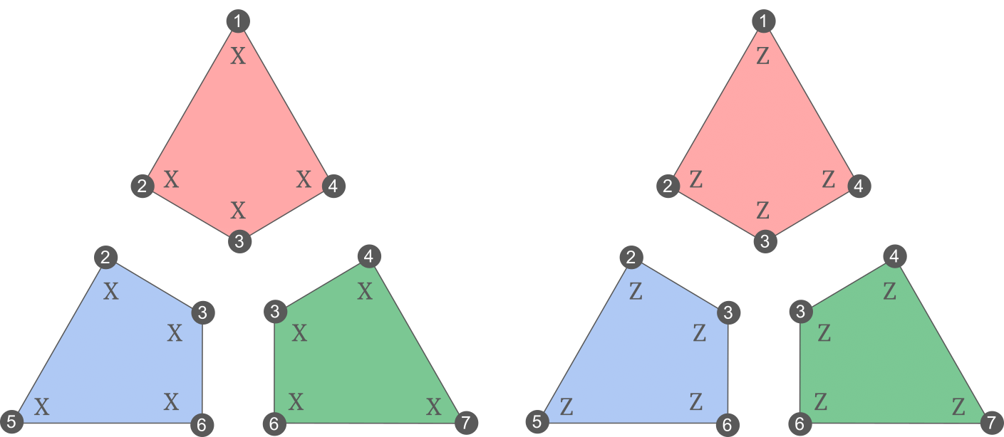
One important thing to notice in the matrix above is that it can be written:

$$\begin{aligned} \bm{H} = \left( \begin{matrix} H_{\text{Hamming}} & \vert & \bm{0} \\ \bm{0} & \vert & H_{\text{Hamming}} \end{matrix} \right) \end{aligned}$$

where $H_{\text{Hamming}}$ is the parity-check matrix of the classical Hamming code.

More generally, the parity-check matrix of any CSS code can be decomposed as

$$\begin{aligned} \bm{H} = \left( \begin{matrix} H_X & \vert & \bm{0} \\ \bm{0} & \vert & H_Z \end{matrix} \right) \end{aligned}$$

where $H_X$ and $H_Z$ are the parity-check matrices of the two classical codes $C_X$ and $C_Z$. The condition that all the $X$ stabilizers should commute with all the $Z$ stabilizers can be written as

$$\begin{aligned} H_X H_Z^T = \bm{0} \end{aligned}$$

Indeed, each component $i,j$ of the product $H_X H_Z^T$ is equal to the dot product (modulo $2$) between the $X$-check $i$ and the $Z$-check $j$. This dot product will be $0$ if and only if the two checks intersect on an even number of bits, or in other words, if the corresponding stabilizers commute.

Even more generally, the parity-check matrix $\bm{H}$ of any stabilizer code must satisfy:

$$\begin{aligned} \bm{H} \odot \bm{H} = \bm{0} \end{aligned}$$

where $\odot$ is the matrix version of the binary symplectic product, defined such that each component $i,j$ is the binary symplectic product between row $i$ of the first matrix and row $j$ of the second matrix. This constraint is what makes it hard to design quantum codes by using classical constructions: most classical codes don’t satisfy this property. But that’s also what makes quantum error correction so unique and interesting, as very specific tools have been introduced in the field in order to come up with new quantum codes. For instance, the topological interpretation of this constraint (as a chain complex) explains the wide intersection between topology and quantum error correction, which doesn’t arise classically. We will start studying topological quantum error correction in the next post, but for now, let’s continue studying the properties of those parity-check matrices.

Syndrome and logical operators

Given an error $\bm{e}$ written in the binary symplectic format, we can obtain the syndrome $\bm{s}$ using

$$\begin{aligned} \bm{H} \odot \bm{e} = \bm{s} \end{aligned}$$

Indeed, each component of the syndrome tells us whether a given stabilizer commutes with the error, i.e. $s_i=0$ if $\bm{e}$ and $\bm{H}_i$ commute, $s_i=1$ if they anticommute. Note that this is the same equation as the classical one, with the matrix product replaced by the symplectic product. Now, we saw that for classical parity-check matrices, we had $\bm{H} \bm{x} = \bm{0}$ for every codeword $\bm{x}$. However, we don’t really have “codewords” in quantum error correction. So what would be the equivalent of $\bm{x}$ in this equation, or in other words, what is the kernel of $\bm{H}$? Any guess?

The kernel of $\bm{H}$ is the set of logical operators! Indeed, as we saw in the first section of this post, we can define logical operators as elements of $\mathcal{C}(\mathcal{S})$, which by definition is the set of all the elements that commute with the stabilizers. And if you remember, this set includes both stabilizers and non-trivial logical operators.

This fact is actually very useful in practice: it gives us a systematic method to find the non-trivial logicals of a given a code. Find a basis for the kernel of $\bm{H}$, and keep all the elements that cannot be written as linear combinations of rows of $\bm{H}$, that is, which are not stabilizers.

Decoding

As for classical error correction, the decoding problem for quantum codes can be expressed using parity-check matrices. However, there is an important subtlety compared to the classical case. Instinctively, we would like to express the decoding problem as follow:

$$\begin{aligned} \max_{\bm{c} \in \mathbb{Z}_2^{2n}} P(\bm{c}) \; \text{ s.t. } \; \bm{H} \odot \bm{c} = \bm{s} \end{aligned}$$

This corresponds to finding the error $c$ that fits the syndrome and has the highest probability of happening. However, the actual goal is not quite exactly that.

To see why, let’s first slightly reformulate the syndrome equation constraint from above. If $\bm{e}$ is the actual error and we choose to apply a correction operator $\bm{c}$, the total operator $\bm{e}+\bm{c}$ applied to the code satisfies:

$$\begin{aligned} \bm{H} \odot (\bm{e} + \bm{c}) = \bm{s} + \bm{s} = \bm{0} \end{aligned}$$

Therefore $\bm{e}+\bm{c} \in \text{Ker}(\bm{H})$ is either a stabilizer or a non-trivial logical operator. If it is a stabilizer, it doesn’t have any effect on the codespace, and mission accomplished. If it is a non-trivial logical operator, we have failed the decoding process and applied a logical error to the state.

Now, let’s notice that if a given correction satisfies the syndrome equation, any stabilizer $\bm{x} \in \mathcal{S}$ applied on top of this correction will also satisfy the syndrome equation:

$$\begin{aligned} \bm{H} \odot (\bm{c} + \bm{x}) = \bm{s} + \bm{0} = \bm{s} \end{aligned}$$

And not only that, but $\bm{e}+(\bm{c}+\bm{x})=(\bm{e}+\bm{c})+\bm{x}$, so the final operators will be the same up to a stabilizer. Therefore, it’s tempting to do as in the previous post and create an equivalence relation between correction operators that fit the syndrome. We say that two operators $\bm{c}$ and $\bm{c'}$ are equivalent if there exists a stabilizer $\bm{x} \in \mathcal{S}$ such that $\bm{c}=\bm{c'}+\bm{x}$. Equipped with this equivalence relation, we can now partition all the correction operators into cosets: two operators belong to the same coset if they are equivalent. And here is the key of the quantum decoding problem: we only need to find a correction operator that belongs to the same coset as the error. Indeed, if $\bm{e}$ and $\bm{c}$ belong to the same coset, it means that there exists $\bm{x} \in \mathcal{S}$ such that $\bm{c}=\bm{e}+\bm{x}$. Therefore, the total operator $\bm{e}+\bm{c}=\bm{e}+\bm{e}+\bm{x}=\bm{x}$ is a stabilizer. On the other hand, if they belong to a different coset, the sum can’t be a stabilizer, since $\bm{e}+\bm{c} = \bm{x}$ for $\bm{x} \in \mathcal{S}$ implies that $\bm{c}=\bm{e}+\bm{x}$ and $\bm{e} \sim \bm{c}$. This means that $\bm{e}+\bm{c}$ is a non-trivial logical operator (i.e. a logical error).

Denoting $\mathcal{E}_{\bm{s}}$ the set of operators that fit the syndrome $\bm{s}$, and $\mathcal{E}_{\bm{s}} / \mathcal{S}$ the set of all cosets (called a quotient space), we can express the real objective of the quantum decoding problem as finding the coset $\bm{\bar{c}} \in \mathcal{E}_{\bm{s}} / \mathcal{S}$ with the highest probability:

$$\begin{aligned} \max_{\bm{\bar{c}} \in \mathcal{E}_{\bm{s}} / \mathcal{S}} P(\bm{\bar{c}}) \end{aligned}$$

where $P(\bm{\bar{c}})$ can be calculated as $P(\bm{\bar{c}}) = \sum_{\bm{c} \in \bm{\bar{c}}} P(\bm{c})$.

For many codes, it’s possible to find syndromes where those two versions of the decoding problem give a different solution. This will be the case when the coset containing the most likely error have much less elements than another coset which contain slightly less likely errors. However, in practice, the two decoding problems often have the same solution, and many practical decoders only seek to solve the first optimization problem. This often results in a small decrease of performance, for a high gain in speed (this is for instance the case of the matching decoder for the surface code, that you might have heard of).

As always, let’s apply what we’ve just learned to the Steane code. As an example, let’s see how to decode a syndrome consisting of a single blue $X$-plaquette. Here are the two cosets of $Z$ operators that fit this syndrome:

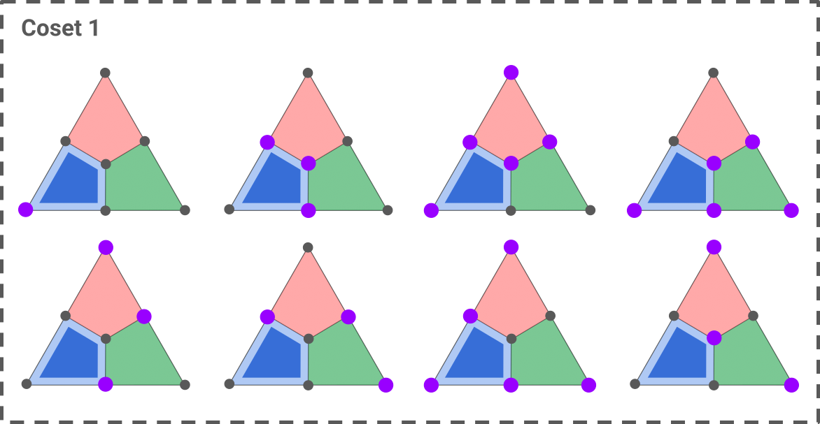
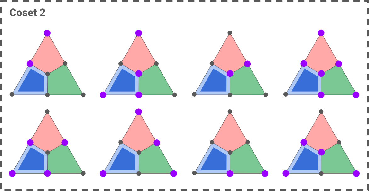
The first coset is constructed by taking the only single-qubit error that fits the syndrome, shown in the top-left triangle, and applying the seven $Z$ stabilizers to it (blue, red, green, blue-red, blue-green, red-green, red-blue-green). The second coset is obtained in a similar way, starting with the two-qubit operator shown in the top-left triangle.

Assuming an i.i.d noise, we can immediately solve the first decoding problem: the most likely error is the one of minimum weight, that is, the first error of coset 1. We can therefore choose any correction operator in this coset as our decoding solution.

Solving the second decoding problem requires a bit more work. Let $p$ the probability that an error occurs on a given qubit, that is, the error rate of the noise channel. Each weight-$k$ error has a probability $\pi_k = p^k (1-p)^{7-k}$. Summing the probabilities of all the elements, we get

$$\begin{aligned} P(\text{coset 1}) &= \pi_1 + 4 \pi_3 + 3 \pi_5 \\ P(\text{coset 2}) &= 3 \pi_2 + 4 \pi_4 + \pi_6 \end{aligned}$$

Plotting those two probabilities as a function of the error rate, we can see that the first coset always has a higher probability than the second one:

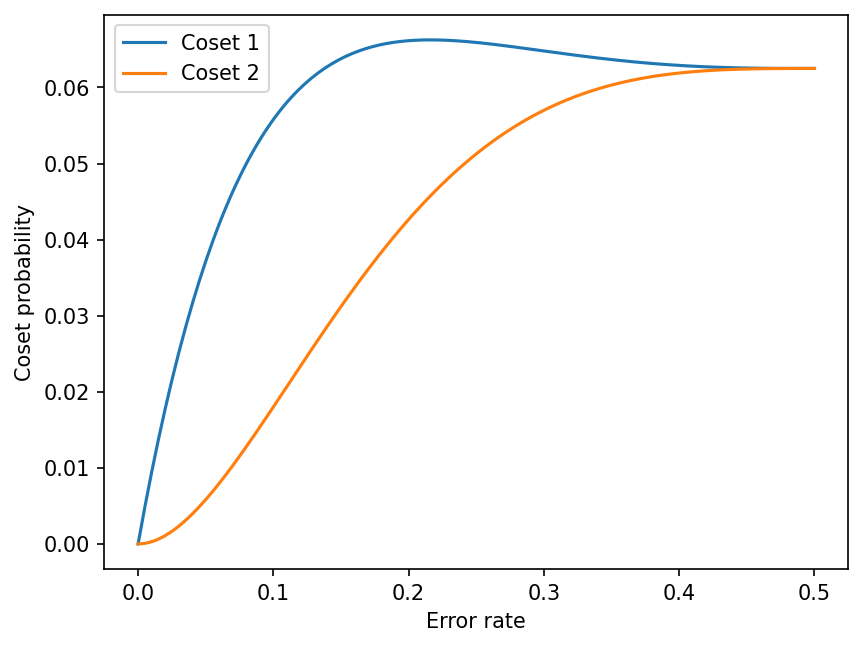
This can also be shown analytically by noticing that⁴

$$\begin{aligned} P(\text{coset 1}) - P(\text{coset 2}) = p (1-p) (1-2p)^3 (2p^2 - 2p + 1) \end{aligned}$$

from which we can deduce that $P(\text{coset 1}) > P(\text{coset 2})$ for $0 < p < \frac{1}{2}$.

Therefore, both decoding formulations give the first coset as our decoding solution.

Tanner graph

Many methods to design quantum codes and decoders work by representing stabilizer codes using their so-called Tanner graph. The Tanner graph of a code associated to an $m \times 2n$ parity-check matrix $H$ is built by creating $2n+m$ nodes: two nodes per qubit (one for $X$ errors and one for $Z$ errors), and one node per stabilizer. By convention, qubit nodes are often represented by circles and stabilizer nodes by squares. Each stabilizer node is then connected to the qubits in its support (with the right Pauli operators). In other words, $H$ is the biadjacency matrix of the Tanner graph.

As an example, here is the Tanner graph of the Steane code, where I colored the stabilizer nodes to indicate to which plaquette operators they correspond.

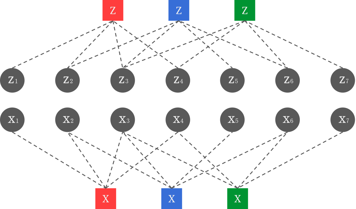
The fact that this graph contains two separate components (the $X$ part and the $Z$ part) is due to the CSS nature of the Steane code. In general, a stabilizer node can be connected to both $X$ and $Z$ qubit nodes.

Many properties of codes and decoders can be interpreted in terms of Tanner graphs. For instance, a low-density parity-check (LDPC) code can be defined as a code whose Tanner graph has constant degree (each qubit is connected to $O(1)$ stabilizers and each stabilizer to $O(1)$ qubits). Similarly, a hypergraph-product code is best interpreted as a certain product of Tanner graphs. Finally, the performance of the belief propagation decoder on a certain code strongly depends on the size of the shortest cycle (also called the girth) of its Tanner graph.

Conclusion

Let’s summarize what we have learned in this post. Pauli operators acting on $n$ qubits can be expressed as binary vectors with $2n$ components: this is the binary symplectic format. The symplectic product on such vectors indicates whether two Pauli operators commute or not. Writing the generators of a stabilizer code in the binary symplectic format gives a parity-check matrix representing the code, and multiplying this parity-check matrix with an error vector gives the syndrome. As a result, logical operators (including stabilizers) are elements of the kernel of the parity-check matrix. To perform decoding, an optimal algorithm should choose a correction operator that belongs to the most likely coset of errors fitting the syndrome. However, decoders that simply output the most likely error often have acceptable performance in practice. Finally, the Tanner graph of a code is the the graph which has the parity-check matrix as its biadjacency matrix.

This is it for the stabilizer trilogy, well done for having read this far! You should now be equipped with all the foundations to start delving into the quantum error correction literature and understand the most popular codes and decoders out there!

While the formalism that we have developed so far is helpful to analyze any code you will encounter, you probably still have no idea how to come up with a new code on your own. The next series of posts will be dedicated to a quite general code construction that builds on top of the stabilizer formalism: topological quantum error correction. So be ready for a new journey towards the surface code and its generalizations!

Solution of the exercise

Exercise: Write the parity-check matrix of Shor’s code (Back to section)

Correction: Shor’s code can be generated by the $Z$-stabilizers $Z_1 Z_2$ and $Z_2 Z_3$ on each 3-qubit block, as well as the $X$-stabilizers $\overline{X_1} \overline{X_2}$ and $\overline{X_2} \overline{X_3}$ (using the notations defined in first post of the series). This gives the following parity-check matrix:

$$\begin{aligned} \bm{H} = \left( \begin{matrix} 1 & 1 & 1 & 1 & 1 & 1 & 0 & 0 & 0 & \vert & 0 & 0 & 0 & 0 & 0 & 0 & 0 & 0 & 0 \\ 0 & 0 & 0 & 1 & 1 & 1 & 1 & 1 & 1 & \vert & 0 & 0 & 0 & 0 & 0 & 0 & 0 & 0 & 0 \\ 0 & 0 & 0 & 0 & 0 & 0 & 0 & 0 & 0 & \vert & 1 & 1 & 0 & 0 & 0 & 0 & 0 & 0 & 0 \\ 0 & 0 & 0 & 0 & 0 & 0 & 0 & 0 & 0 & \vert & 0 & 1 & 1 & 0 & 0 & 0 & 0 & 0 & 0 \\ 0 & 0 & 0 & 0 & 0 & 0 & 0 & 0 & 0 & \vert & 0 & 0 & 0 & 1 & 1 & 0 & 0 & 0 & 0 \\ 0 & 0 & 0 & 0 & 0 & 0 & 0 & 0 & 0 & \vert & 0 & 0 & 0 & 0 & 1 & 1 & 0 & 0 & 0 \\ 0 & 0 & 0 & 0 & 0 & 0 & 0 & 0 & 0 & \vert & 0 & 0 & 0 & 0 & 0 & 0 & 1 & 1 & 0 \\ 0 & 0 & 0 & 0 & 0 & 0 & 0 & 0 & 0 & \vert & 0 & 0 & 0 & 0 & 0 & 0 & 0 & 1 & 1 \end{matrix} \right) \end{aligned}$$

1. See for instance belief propagation defined over GF(4) ↩︎

2. qecsim, PanQEC, PyMatching, ldpc, etc. ↩︎

3. If you know a bit of abstract algebra, you will notice that our map defines an isomorphism from the Pauli group (modulo the phase) to the group $(\mathbb{Z}_2^2, +)$ ↩︎

4. Thanks Alex Cliffe for suggesting this proof! ↩︎