The stabilizer trilogy I — Stabilizer codes
Now that you know all you need to know about classical error correction, the time has finally come to learn how to correct those damn errors that keep sabotaging your quantum computer! The key tool, introduced by Daniel Gottesman in his landmark 1997 PhD thesis is the stabilizer formalism. The same way most classical codes fall into the linear code category, almost all the quantum codes you will encounter can be classified as stabilizer codes. And for a good reason: stabilizer codes are simply the quantum generalization of linear codes! Your beloved parity checks will turn into stabilizers, a set of commuting measurements controlling the parity of your qubits in different bases. Parity-check matrices and Tanner graphs will get slightly bigger and more constrained. But apart from that, if you’re more or less comfortable with the notions discussed in the last post, going quantum shouldn’t give you too much trouble.
So, what’s the plan? To make the content of this post a bit more digestible, I’ve decided to divide it into three parts: the stabilizer trilogy. In the first part, we will start by motivating the need for the stabilizer formalism, using the quantum repetition code and Shor’s code as examples. We will then be ready to formally define stabilizer codes and one of its most important families, the CSS codes. To illustrate our construction, we will end the post by introducing a simple code that really exemplifies the stabilizer and CSS construction: the Steane code. Finally, in case you need it, I’ve put some reminders on the manipulation of Pauli operators in the appendix.
In the second part of this series, we will look more deeply into the properties of stabilizer codes. In particular, we will introduce the notion of logical operator, and see how it can be used to derive the parameters of stabilizer codes. In the last part, we will learn how to generalize parity-check matrices and Tanner graphs to the quantum setting. This formulation can be used to express the decoding problem formally and to implement quantum code simulation in practice.
This trilogy should give you all you need to start exploring the quantum error correction literature. And with all those tools in our hand, we will finally be ready to study one of the most popular quantum code: the surface code! So hang in there, have a good read, and I assure you the journey will be worth it!
Motivation: a new lens on the quantum repetition code
To understand the challenges in building quantum codes, let’s look back at our good ol’ quantum repetition code (introduced in the first post of this series), with our new error correction knowledge. As a reminder, the quantum repetition code is defined as the encoding of a single-qubit logical state \(\vert \psi \rangle_L = a \vert 0 \rangle_L + b \vert 1 \rangle_L\) as a 3-qubit physical state:
\[\begin{aligned} \vert \psi \rangle = a \vert 000 \rangle + b \vert 111 \rangle \end{aligned}\]We define the codespace of our code as the space of all the states that can be written as above (for any \(a,b\)). Let’s see how errors affect the codespace. As we saw in the first post, quantum noise comes into two flavours: \(X\) errors, also known as bit flips, and \(Z\) errors, also known as phase flips. Let’s focus on \(X\) errors first. If an \(X\) error occurs on the first qubit, the state is transformed into
\[\begin{aligned} \vert \widetilde{\psi} \rangle = X_1 \vert \psi \rangle = a \vert 100 \rangle + b \vert 011 \rangle \end{aligned}\]In the classical repetition code, errors such as this one could be detected by reading the message and seeing that it is neither \(000\) or \(111\), or in other words, it is not a codeword. Decoding would then consist of taking a majority vote on the three bits.
However, in the quantum case, “reading the message” would collapse the state and ruin any further computation we might want to do on this state. To make error detection work, let’s remember that there is another technique to detect errors on linear codes (including the repetition code), that we saw in the last post: we can look at the parity checks of the code! For the classical repetition codes, those parity checks measured the parity of all the pairs of bits. If some of the checks had an odd parity, it meant that an error had occurred, and depending on which pairs had a violated parity-check equation, we could then decode any single bit-flip error.
And that’s where the magic comes in: those parity checks can be measured quantumly without collapsing the state! First, you might wonder what “parity” means for our state, given that we have a superposition of two computational basis elements in the codespace. However, it’s easy to verify that it is actually well-defined. Consider the state \(\vert \psi \rangle\) subjected to any number of bit-flip errors. Choose one of the two elements of the superposition. Look at the parity of a pair of qubits. This parity will be the same if you had chosen the other element of the superposition. This is due to the fact that bit flips are always applied simultaneously on both parts of the superposition.
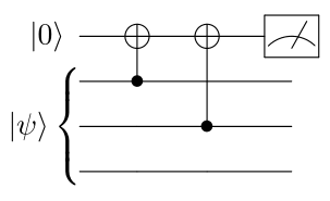
Now, how do we measure this parity? We can simply measure the observable \(Z_i Z_j\). Indeed, \(\vert \psi \rangle\) is an eigenstate of \(Z_i Z_j\), and remains so when bit-flip errors are applied to the state. For instance, \(Z_1 Z_2 \vert \psi \rangle = \vert \psi \rangle\), meaning that measuring \(Z_1 Z_2\) on the error-free state will give \(+1\). On the other hand, \(Z_1 Z_2 \vert \widetilde{\psi} \rangle = Z_1 Z_2 X_1 \vert \psi \rangle = - X_1 Z_1 Z_2 \vert \psi \rangle = -\vert \widetilde{\psi} \rangle\), so measuring this operator when a bit-flip has occurred on the first qubit gives \(-1\) (if this manipulation of Pauli operators is not straightforward to you, feel free to read the Appendix on Pauli operators and come back). Checking those calculations on your own, and for other examples of bit-flip errors, should convince you that measuring \(Z_i Z_j\) gives you exactly the parity between the qubits \(i\) and \(j\). In general, the result of measuring those operators is exactly like the syndrome we introduced in the previous post: we get \(+1\) when a parity-check equation is satisfied, and \(-1\) when it is not. As an example of how to measure those parity checks, the circuit to measure \(Z_1 Z_2\) is given below:
So, what have we done so far? We have found a set of operators \(\{Z_i Z_j\}\) such that:
- Our error-free state is a simultaneous \(+1\) eigenstate of all those operators
- Single and two-qubit \(X\) errors anti-commute with some of them, allowing the detection and correction of \(X\) errors.
We will soon call those operators “stabilizers”, and study their general properties. But first—you might have been wondering all this time—what about \(Z\) errors? As it happens, they are actually undetectable by our code. For instance, if a \(Z\) error were to occur on the first qubit of the state \(\vert \psi \rangle\), we would get the state
\[\begin{aligned} \vert \widetilde{\psi} \rangle = Z_1 \vert \psi \rangle = a \vert 000 \rangle - b \vert 111 \rangle \end{aligned}\]This is still in the codespace of our code! Therefore, we have no way to detect this error: \(Z\) errors are logical errors. We define the distance of a code as the smallest Pauli error that maps the codespace to itself, or in other words, the smallest logical error. Since a single \(Z\) error in the quantum repetition code is undetectable, it means that the distance of the code is \(1\). Denoting \(n\) the number of physical qubits of a code, \(k\) the number of logical qubits it encodes, and \(d\) its distance, we say that the repetition code is an \([[n,k,d]]=[[n,1,1]]\)-code. Note the use of double brackets, a common convention used to distinguish quantum from classical codes.
So what do we do from there? Taking inspiration from the quantum repetition code, let’s try to build our first code that can detect both \(X\) and \(Z\) errors: Shor’s code.
Our first truly quantum code: Shor’s code
To understand the idea behind Shor’s code, let’s first see how we could design a repetition code that only protects information against \(Z\) errors, instead of \(X\) errors. Can you see what modification of the repetition code would be required?
The idea is to simply use a different basis for the codewords. Indeed, replacing \(\{\vert 000\rangle, \vert 111\rangle\}\) by \(\{\vert +++\rangle, \vert ---\rangle\}\), and the parity-check measurements \(\{Z_i Z_j\}\) by \(\{X_i X_j\}\), we obtain a code that can correct any single-qubit \(Z\) error.
The trick found by Peter Shor is to combine those two codes using a process called concatenation. It consists of encoding the logical qubits of one code using a second code. In our case, we can encode the logical qubits of the \(Z\)-basis repetition code into the \(X\)-basis repetition code. This defines the 9-qubit Shor’s code, made of the following codewords
\[\begin{aligned} \vert 0 \rangle_{L_2} = \vert + \rangle_{L_1} \otimes \vert + \rangle_{L_1} \otimes \vert + \rangle_{L_1} = \frac{1}{2^{3/2}} \left(\vert 000 \rangle + \vert 111 \rangle \right) \left(\vert 000 \rangle + \vert 111 \rangle \right) \left(\vert 000 \rangle + \vert 111 \rangle \right) \\ \vert 1 \rangle_{L_2} = \vert - \rangle_{L_1} \otimes \vert - \rangle_{L_1} \otimes \vert - \rangle_{L_1} = \frac{1}{2^{3/2}} \left(\vert 000 \rangle - \vert 111 \rangle \right) \left(\vert 000 \rangle - \vert 111 \rangle \right) \left(\vert 000 \rangle - \vert 111 \rangle \right) \end{aligned}\]where \(\vert \cdot \rangle_{L_1}\) refers to logical qubits after the first encoding, for which \(\vert 0 \rangle_{L_1}=\vert 000 \rangle\), and \(\vert \cdot \rangle_{L_2}\) refers to logical qubits after the second encoding, for which \(\vert 0 \rangle_{L_2}=\vert +++ \rangle_{L_1}\).
Now, if an \(X\) error occurs on any of the 9 qubits, we will be able to correct it by measuring \(Z_i Z_{j}\) on all the qubits \(i\) and \(j\) of the same block. Indeed, you can check that in the absence of error, we have
\[\begin{aligned} Z_i Z_j \vert \psi \rangle_{L_2} = \vert \psi \rangle_{L_2} \end{aligned}\]with \(\vert \psi \rangle_{L_2} = a \vert 0 \rangle_{L_2} + b \vert 1 \rangle_{L_2}\). This means that measuring those operators will give the result \(+1\).
On the other hand, let’s say we have an \(X\) error on the fourth qubit of the logical zero state. It would result in the state:
\[\begin{aligned} X_4 \vert 0 \rangle_{L_2} = \frac{1}{2^{3/2}} \left(\vert 000 \rangle + \vert 111 \rangle \right) \left(\vert 100 \rangle + \vert 011 \rangle \right) \left(\vert 000 \rangle + \vert 111 \rangle \right) \end{aligned}\]The odd parity between qubit 4 and qubits 5 and 6, detected by measuring \(Z_4 Z_5\) and \(Z_5 Z_6\), tells us that the \(X\) error occurred on qubit \(4\). We can therefore correct this error, and more generally any other single-qubit \(X\) error, by analyzing the result of the \(Z_i Z_j\) measurements.
Let’s now focus our attention to \(Z\) errors. Let’s remember that for the Z-basis repetition code, the operator \(\overline{X}=XXX\) is a logical Pauli \(X\) operator, turning \(\vert 0 \rangle_{L_1}\) into \(\vert 1 \rangle_{L_1}\). Let’s write \(\overline{X_1}=X_1 X_2 X_3\), \(\overline{X_2}=X_4 X_5 X_6\) and \(\overline{X_3}=X_7 X_8 X_9\).
To detect \(Z\) errors, we can measure the parity \(\overline{X}_i \overline{X}_{j}\) for all \(i,j \in \{1,2,3\}\), \(i \neq j\). Indeed, you can verify explicitly that we have
\[\begin{aligned} \overline{X_i} \overline{X_j} \vert \psi \rangle_{L_2} = \vert \psi \rangle_{L_2} \end{aligned}\]for all \(i,j\). Moreover, if a \(Z\) error occurs, for example on the fourth qubit of the logical zero state, we would get:
\[\begin{aligned} Z_4 \vert 0 \rangle_{L_2} = \vert +-+ \rangle_{L_1} = \frac{1}{2^{3/2}} \left(\vert 000 \rangle + \vert 111 \rangle \right) \left(\vert 000 \rangle - \vert 111 \rangle \right) \left(\vert 000 \rangle + \vert 111 \rangle \right) \end{aligned}\]The odd parity between blocks \(1\) and \(2\) and blocks \(2\) and \(3\) can be detected using the operator \(\overline{X_1} \overline{X_2} = X_1 X_2 X_3 X_4 X_5 X_6\) and \(\overline{X_2} \overline{X_3} = X_4 X_5 X_6 X_7 X_8 X_9\). You can check that explicitly by applying those operators to \(Z_4 \vert 0 \rangle_{L_2}\) and showing for instance that
\[\begin{aligned} \overline{X_1} \overline{X_2} Z_4 \vert 0 \rangle_{L_2} = - Z_4 \vert 0 \rangle_{L_2} \end{aligned}\]meaning that the result of measuring \(\overline{X_1} \overline{X_2}\) will be \(-1\). Similarly, the result of measuring \(\overline{X_2} \overline{X_3}\) will be \(-1\). However, note that we would have obtained the exact same measurement result if the \(Z\) error had occurred on qubit \(5\) or qubit \(6\). That’s our first example of error degeneracy: different errors causing the same syndrome. How do we decide where to apply our correction then? The answer is that it doesn’t matter: we can choose either of the three middle qubits. To see why, let’s look at what happens if we apply \(Z_5\) to a state affected by the error \(Z_4\):
\[\begin{aligned} Z_5 Z_4 \vert \psi \rangle_{L_2} = \vert \psi \rangle_{L_2} \end{aligned}\]It gets us back to the original state! The reason is that any state in the codespace is a +1 eigenstate of \(Z_5 Z_4\) (as we saw when looking at \(X\) error detection). The same phenomenon would have happened if we had applied \(Z_6\), and therefore we can correct the \(Z_4\) error by applying a \(Z\) operator on any of the three middle qubits. More generally, any single-qubit \(Z\) error can be corrected by analyzing the result of the \(\overline{X}_i \overline{X}_{j}\) measurements. This trick for dealing with error degeneracies is preponderant in quantum error correction, and we will see the most general version of it when looking at decoding stabilizer codes (in the next post).
So our code is able to detect and correct any single-qubit error. But what about errors of higher weight? Or in other words, what is the distance of Shor’s code (i.e. the smallest undetectable errors)? Since this is a perfect exercise to see if you’ve understood this code, I leave this question as an exercise!
In summary, we have found a \([[9,1,3]]\) quantum code that can detect both \(X\) and \(Z\) errors by measuring a set of operators \(\{ Z_i Z_j \}\) and \(\{\overline{X_i} \overline{X_j} \}\). This means that error-free states (i.e. codewords) are a common \(+1\) eigenstate of those operators, while states subjected to weight-1 and weight-2 errors are \(-1\) eigenstates of some of those operators, allowing us to detect those errors. With this example in mind, we are now finally ready to delve into the stabilizer formalism!
Stabilizer formalism: first definitions
The stabilizer formalism allows us to generalize the ideas above in order to come up with new quantum codes and study their properties. The main idea is to change our perspective from states (or codewords) to operators, similarly to the way we defined classical linear codes using parity-check matrices. But generalizing parity-check operators in the quantum setting requires a bit of care. Let’s see how it works.
First, let me outline the general idea of this section. As we saw with Shor’s code, errors in a quantum code can be detected by measuring a certain set of operators, generalizing the parity checks of classical codes. Those operators are called stabilizers and have a certain number of properties: they have eigenvalues \(+1\) and \(-1\), they all commute (the order of measurement doesn’t matter), etc. Moreover, any codeword is a common \(+1\) eigenstate of all the stabilizers, i.e. measuring any stabilizer on an error-free state gives the value \(+1\) and does not disturb the state.
The goal is to go backward: given any set of stabilizers, does it define a code? As found out by Daniel Gottesman, the answer is yes, and this simple fact has been foundational for quantum error correction, allowing us to find codes by searching for stabilizers with good properties. Let us now introduce the formalism behind this brilliant idea.
The n-qubit Pauli group \(\mathcal{P}_n\) is the set of all Pauli operators on \(n\) qubits, with the usual matrix multiplication as the group operation, that is:
\[\begin{aligned} \mathcal{P}_n=\{ \omega P_1 \otimes \ldots \otimes P_n : P_i \in \{I,X,Y,Z \}, \omega \in \{1,-1,i,-i\}\} \end{aligned}\]Note that the phase factor is included in order for this set to be close under the group operation.
We can now define a stabilizer group as an abelian subgroup of the Pauli group that does not contain \(-I\). Let’s slowly break that down. First, the stabilizer group is a subgroup of the Pauli group, meaning that every element is a Pauli operator, and has in consequence eigenvalues \(+1\) and \(-1\). It is a group, meaning that the product of any two stabilizers is also a stabilizer. This group is abelian, meaning that any two stabilizers commute, and can therefore be measured in any order. Finally, we don’t want \(-I\) to be included, or equivalently we don’t want any two operators \(S\) and \(-S\) to be in the same stabilizer group, as it will make sense shortly.
We can now define a stabilizer code as the common \(+1\) eigenspace of all the operators in a stabilizer group. That is, given a stabilizer group \(\mathcal{S}\), we define the codespace of a stabilizer code as:
\[\begin{aligned} \mathcal{C}=\{ \vert \psi \rangle : S\vert \psi \rangle = \vert \psi \rangle, \forall S \in \mathcal{S} \} \end{aligned}\]This set is well-defined, since by definition all the stabilizers commute, and have therefore some common eigenstates. Moreover, each stabilizer has at least one \(+1\) eigenvalue (remember that \(-I\) is not included in the stabilizer group), so there is a common \(+1\) eigenstate of all the stabilizers. Finally, you can notice that \(\mathcal{C}\) forms a vector space, and therefore defines a valid code.
This one-to-one correspondence between codespaces defined as above and stabilizer groups is the foundation of quantum error correction: instead of the thinking of codes in the state picture (as a vector space of states), we can now think of them in the operator picture (as a stabilizer group). For instance, Shor’s code can either be defined in the state picture, as the codespace \(\{a \vert 0 \rangle_{L_2} + b \vert 1 \rangle_{L_2} \}\) (with \(\vert 0 \rangle_{L_2}\) and \(\vert 1 \rangle_{L_2}\) defined in the previous section), or in the operator picture, as the codespace stabilized by \(\langle Z_i Z_j, \overline{X_i} \overline{X_j} \rangle\) with \(i,j\) neighboring physical/logical qubits.
Last but not least, how can we detect and correct errors with a stabilizer code? As we saw with the repetition code and Shor’s code, the idea is to simply measure all the stabilizers, resulting in what is called the syndrome. If no error has occurred, the syndrome should consist of \(+1\) for all the stabilizers. If a Pauli error \(E\) has occurred, there are two possibilities for each stabilizer \(S\): either it commutes or it anticommutes with it. If it commutes, we will measure \(+1\):
\[\begin{aligned} SE \vert \psi \rangle = ES \vert \psi \rangle = E \vert \psi \rangle \end{aligned}\]If it anticommutes, we will measure \(-1\):
\[\begin{aligned} SE \vert \psi \rangle = - ES \vert \psi \rangle = - E \vert \psi \rangle \end{aligned}\]To detect \(X\) errors, we therefore need stabilizers with some \(Z\) or \(Y\) operators, while to detect \(Z\) errors, we need stabilizers with some \(X\) or \(Y\) operators.
By analyzing the syndrome, it is often possible to correct errors as well. However, one specificity of quantum codes is that we often don’t need to find the exact qubits on which the errors have occurred. What we need is to find a correction operator \(C\) that restores our state, that is:
\[\begin{aligned} C E \vert \psi \rangle = \vert \psi \rangle \end{aligned}\]In other words, we want \(C E\) to be a stabilizer. For instance, in Shor’s code, we saw that if the error \(Z_4\) occurs, we can correct it by using either \(Z_4\), \(Z_5\) or \(Z_6\) as our correction operator. This was due to \(Z_4 Z_4\), \(Z_4 Z_5\) and \(Z_4 Z_6\) being stabilizers. Finding the best correction operator is the essence of the decoding problem, which we will see in more details in the next post.
So what have we done so far? We have shown that given a stabilizer group, that is a set of commuting Pauli operators that does not contain \(-I\), we can construct a quantum code by considering the common +1 eigenspace of all the stabilizers. When errors occur in this code, moving the state outside of the codespace, they can be detected (and sometimes corrected) by measuring all the stabilizers and checking if some measurements are equal to \(-1\).
However, we haven’t yet given any method to construct interesting stabilizer groups. The next section introduces one of the most important family of stabilizer codes, the CSS codes, which will help us to build a new example of quantum code: the quantum version of the Hamming code.
Quantum codes from classical codes: the CSS construction
So, how can we construct stabilizer codes? One method is to start from two classical codes: one that will take care of \(X\) errors and one that will take care of \(Z\) errors. As we saw in the previous section, to correct \(X\) errors, we can use stabilizers made of \(Z\) operators, and to correct \(Z\) errors, we can use stabilizers made of \(X\) operators.
The idea is therefore the following: let’s pick two classical codes that we will call \(C_X\) and \(C_Z\). For each parity check of \(C_X\), supported on bits \(b_1,\ldots,b_k\), add the stabilizer \(X_{b_1} \ldots X_{b_k}\) to the stabilizer group. Similarly, for each parity check of \(C_Z\), supported on bits \(b'_1,\ldots,b'_k\), add the stabilizer \(Z_{b'_1} \ldots Z_{b'_k}\) to the stabilizer group. For the resulting quantum code to be valid, remember that all the stabilizers should commute. While stabilizers of the same Pauli type necessarily commute, it is not obvious that all the \(Z\) stabilizers commute with all the \(X\) stabilizers. For this to be the case, each \(X\) stabilizer should intersect on an even number of qubits with all the \(Z\) stabilizers (see Appendix).
If this is the case, the resulting quantum code is valid and form what is called a Calderbank-Shor-Steane (CSS) code. More precisely, a CSS code is a stabilizer code that can be generated by a set of pure \(X\) and pure \(Z\) stabilizers. For instance, both codes that we have encountered before, Shor’s code and the quantum repetition code, are examples of CSS codes. And so are most of the codes that you will encounter in the literature, making CSS codes one of the most important family of codes.
However, if you try the construction above with some random codes \(C_X\) and \(C_Z\) taken from the classical literature, you will find that it is very difficult to pass the commutation criterion. Therefore, more involved methods are needed to construct quantum codes, such as topological constructions or hypergraph products. However, there is on example where our procedure works extremely well: our good old Hamming code!
Steane code, the quantum version of the Hamming code
It’s finally time to illustrate the stabilizer formalism with a concrete example! If the two previous sections were feeling a bit abstract, this section should hopefully clarify things.
So let’s apply the CSS construction to the Hamming code that we introduced in the previous blog post. As a reminder, the Hamming code is a \([7,4,3]\)-code defined by the following three parity check equations1
\[\begin{aligned} x_1 + x_2 + x_3 + x_4 = 0 \\ x_2 + x_3 + x_5 + x_6 = 0 \\ x_3 + x_4 + x_6 + x_7 = 0 \end{aligned}\]Let’s now apply the CSS construction with \(C_X\) and \(C_Z\) two Hamming codes. To \(C_X\), we associate the group \(\mathcal{S}_X\) on 7 qubits defined as:
\[\begin{aligned} \mathcal{S}_X = \langle X_1 X_2 X_3 X_4, X_2 X_3 X_5 X_6, X_3 X_4 X_6 X_7 \rangle \end{aligned}\]and to \(C_Z\), the group \(\mathcal{S}_Z\) defined as:
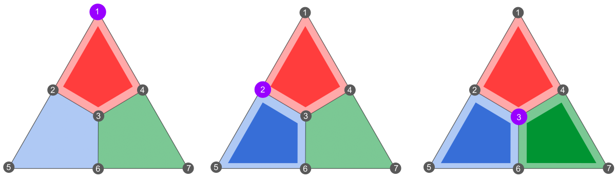
\[\begin{aligned} \mathcal{S}_Z = \langle Z_1 Z_2 Z_3 Z_4, Z_2 Z_3 Z_5 Z_6, Z_3 Z_4 Z_6 Z_7 \rangle \end{aligned}\]It is often convenient to visualize stabilizer codes using some graphical representations. Here is how to visualize the stabilizers defined above:
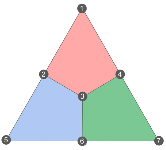
In this figure, each vertex (numbered from 1 to 7) represents a qubit, and each coloured face (often called plaquette in the literature) supports an \(X\) and a \(Z\) stabilizer. The different plaquette stabilizers are shown explicitly here:
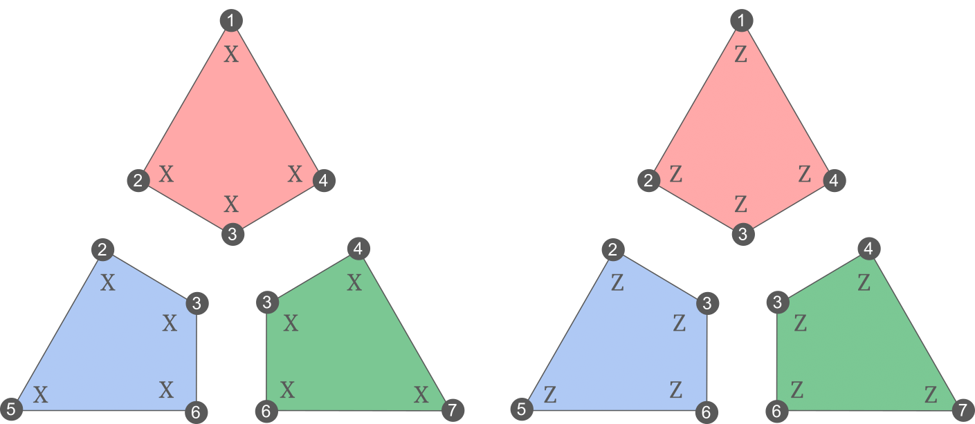
From this representation, it is easy to see that each plaquette stabilizer intersects with every other plaquette stabilizers on exactly two qubits, which is an even number. As we discussed earlier, it means that elements of \(\mathcal{S}_X\) and \(\mathcal{S}_Z\) commute, and we can form a valid code by combining the generators of the two groups. The resulting code is called the Steane code, and is an example of color code (a very interesting family of codes which would deserve their own blog post).
The Steane code is often considered a promising candidate for near-term quantum error correction and is indeed one of the first codes to have been implemented on a real device (by different teams of ion trappers) 2. This is due to its many nice properties: its small size (it only requires \(7\) physical qubits), its 2D locality (it can be built on a 2D lattice without requiring long-range connections to measure the stabilizers), and the presence of many transversal logical gates (a topic for another time). Furthermore, it only requires the measurement of weight-4 stabilizers, as opposed to Shor’s code which requires measuring weight-6 stabilizers. Since errors can happen during the measurement of stabilizers, a good rule of thumb to get well-performing quantum codes is to always try to minimize the weight of its stabilizer generators.
We will study the characteristics of the Steane code in the next post, showing that it is a \([[7,1,3]]\) quantum code. Meanwhile, we can already look at what happens in the presence of single-qubit errors. Since \(X\) and \(Z\) errors are detected in the same way (using either \(X\) or \(Z\) stabilizers on the plaquettes), we can consider the effect of \(Z\) errors only, without loss of generality. Below is the observed syndrome for a single \(Z\) error on qubits \(1\) to \(3\):
In this figure, the purple vertices correspond to \(Z\) errors, and the highlighted plaquettes to stabilizer measurements of \(-1\). To obtain this this result, note that a single-qubit \(Z\) error will always anticommute with the \(X\) plaquette it touches (you can easily show this using the property of the appendix).
You can continue this exercise with the remaining single-qubit errors, and you will see that they all lead to a different syndrome. Therefore, the Steane code can correct any single-qubit error.
Conclusion
In this post, we have introduced the most important tool to build and analyze quantum codes: the stabilizer formalism. Starting from a stabilizer group (set of commuting Pauli operators), we found that we can construct a codespace by considering the common \(+1\) eigenspace of its elements. We defined the family of CSS codes, whose stabilizer generators can be split into pure \(X\) and pure \(Z\) elements. We studied a few examples of stabilizer codes: the \([[3,1,1]]\) repetition code, the \([[9,1,3]]\) Shor code, and the \([[7,1,3]]\) Steane code.
In the next post, we will go further in our study of stabilizer codes: we will learn how to find the logical operators, the distance and the number of encoded qubits of a code. The Steane code will continue to serve as our main example throughout the next post.
Appendix: useful tricks to manipulate Pauli operators
For the discussion that follows, let’s define a Pauli operator as an operator of the form \(P_1 \otimes \ldots \otimes P_n\) with \(P_i \in \{I, X, Y, Z\}\) for all \(i\). As a reminder, here is the definitions of the Pauli matrices \(X,Y,Z\):
\[\begin{aligned} X = \left( \begin{matrix} 0 & 1 \\ 1 & 0 \end{matrix} \right), \; Y = \left( \begin{matrix} 0 & -i \\ i & 0 \end{matrix} \right), \; Z = \left( \begin{matrix} 1 & 0 \\ 0 & -1 \end{matrix} \right) \; \end{aligned}\]We say that two Pauli operators \(P\) and \(P'\) commute if \(P P' = P'P\), and anticommute if \(P P' = -P' P\). The goal of this section is to prove the following extremely useful fact about Pauli operators:
For instance, \(X_1 Y_2 Z_3 X_4\) and \(X_1 Z_4\) anticommute: they intersect on qubits \(1\) (with the same Pauli) and \(4\) (with a different Pauli), so only on one qubit with a different Pauli. On the other hand, \(X_1 X_2 X_3\) and \(Z_2 Z_3 Z_4\) commute as they intersect on two terms (qubits \(2\) and \(3\)) with a different Pauli.
This property is used all the time in quantum error correction: to check that the stabilizers of a code commute, to see how errors affect the stabilizer measurements, etc. So it’s worth getting comfortable with it early in your QEC journey.
So let’s show this fact. Let \(P=P_1 \ldots P_n\) and \(P'=P'_1 \ldots P'_n\) two Pauli operators, with each \(P_i\) and \(P'_i\) acting on qubit \(i\). Our objective is to go from \(PP'=P_1 \ldots P_n P'_1 \ldots P'_n\) to \(P'P=P'_1 \ldots P'_n P_1 \ldots P_n\). For that, we will move each term \(P'_i\) to the top. Since any \(P'_i\) commute with all the terms \(P_j\) with \(i \neq j\) (they act on different qubits), we can move it next to \(P_i\):
\[\begin{aligned} PP'=P_1 \ldots P_i P'_i P_{i+1} \ldots P_n P'_1 \ldots P'_{i-1} P'_{i+1} \ldots P_n \end{aligned}\]Now, if \(P\) and \(P'\) don’t intersect on qubit \(i\), that is either \(P_i=I\) or \(P'_i = I\), we will have \(P_i P'_i = P'_i P_i\). Same result if \(P_i = P'_i\). In those two cases, we can move \(P'_i\) to the top without introducing any minus sign:
\[\begin{aligned} PP'=P'_i P_1 \ldots P_n P'_1 \ldots P'_{i-1} P'_{i+1} \ldots P_n \end{aligned}\]On the other hand, if \(P_i \neq P'_i \neq I\), we will have \(P_i P'_i = - P'_i P_i\) (remember that \(XZ+ZX=XY+YX=YZ+ZY=0\)). This means that moving \(P'_i\) to the top introduces a minus sign:
\[\begin{aligned} PP'=-P'_i P_1 \ldots P_n P'_1 \ldots P'_{i-1} P'_{i+1} \ldots P_n \end{aligned}\]Therefore, each intersection with a different Pauli element introduces a minus sign, and the overall sign will be \(+1\) if and only if there is an even number of such intersections, which proves our propositions.
Solution of the exercise
-
Note that I’m using a different notation from the previous post, giving variables a more generalizable name. If that confuses you, here is the exact mapping: \(z_1 \rightarrow x_1\), \(z_2 \rightarrow x_5\), \(z_3 \rightarrow x_7\), \(a \rightarrow x_2\), \(b \rightarrow x_3\), \(c \rightarrow x_6\), \(d \rightarrow x_4\). ↩︎
-
The \(\vert 0 \rangle_{L}\) state of the Steane code was first implemented by an Austrian team, in Nigg et al., 2014. Actual error correction using stabilizer measurements was then done by Honeywell in Ryan-Anderson et al., 2021. ↩︎