The maths behind topological quantum error correction
To pursue our quantum error correction journey, we now need to dive deeper into the maths that underlie the main ideas of the field! Why \(k\) in the surface code is independent on the specific cellulation.
We will see chain complexes, homological algebra, etc.
All codes are topological codes via code-to-manifold mapping (but not necessarily the natural way to see them). Most codes build on homological ideas.
Motivation
In Part III of the stabilizer trilogy, we saw that CSS codes can be characterized by two matrices, the parity-check matrices \(H_X\) and \(H_Z\), whose rows encode all the \(X\) and \(Z\) stabilizers of the code as binary vectors. For those two matrices to form a valid stabilizer code, we saw that they must obey the condition
\[\begin{aligned} H_X H_Z^T = 0 \end{aligned}\]which means that every \(X\) stabilizer must commute with every \(Z\) stabilizer. Furthermore, the parameters of the code can also be expressed using those matrices. For instance, the number of logical qubits \(k\) is exactly the dimension of the quotient space \(\ker(H_X)/\Im(H_Z^T)\). Why is that so? The kernel of \(H_X\) is the set of Pauli operators that commute with all the \(X\) stabilizers, that is, the set of (trivial and non-trivial) \(Z\) logical operators. And \(\Im(H_Z^T)\) is the set of \(Z\) stabilizers. The quotient therefore represents the equivalence classes of \(Z\) logicals up to stabilizers, which contains one element per logical qubit of the code. Another way to see it is via the formula
\[\begin{aligned} \dim \left( \ker(H_X) / \Im(H_Z^T) \right) = \dim(\ker(H_X)) - \dim(\Im(H_Z^T)) \end{aligned}\]Using the rank-nullity theorem, this gives us
\[\begin{aligned} \dim \left( \ker(H_X) / \Im(H_Z^T) \right) = n - \rank(H_X) - \rank(H_Z^T) \end{aligned}\]where \(\rank(H_X)=\rank(H_X^T)\) is the number of independent \(X\) stabilizers, and \(\rank(H_Z^T)\) is the number of independent \(Z\) stabilizers. This means that
\[\begin{aligned} \dim \left( \ker(H_X) / \Im(H_Z^T) \right) = n - m = k \end{aligned}\]with \(m\) the total number of independent stabilizers, and where we used the formula for the number of logical qubits that we saw in Part II of the stabilizer trilogy.
What about the distance? The \(X\) distance \(d_X\) can be expressed as
\[\begin{aligned} d_X = \min_{L \in \ker(H_Z) \setminus \Im(H_X^T)} |L| \end{aligned}\]and similarly for the \(Z\) distance \(d_Z\). The total distance is then the minimum of \(d_X\) and \(d_Z\).
One last important property that can be read from the parity-check matrices is the locality of the code. It is not enough for a code to have good \([[n,k,d]]\) parameters, it must also have a good fault-tolerant implementation, that is, a set of circuits to extract the syndrome, to prepare the initial states, to perform logical gates, etc. such that the threshold is non-zero (i.e. there exists a non-zero physical error rate under which scaling the code and the corresponding circuits exponentially decreases the logical error-rate). One sufficient condition for a code family with growing distance to possess such fault-tolerant implementation is for it to be a low-density parity-check (LDPC) code: each stabilizer must be attached to a constant number of qubits, and each qubit to a constant number of stabilizers. This was for instance shown in a classic 2013 paper by Daniel Gottesman. From the point-of-view of our matrices, a code family with parity-check matrices \((H_X,H_Z)\) is LDPC if both \(H_X\) and \(H_Z\) are sparse, that is, the weight of their rows and columns is constant when increasing the size of the code1.
Where does this lead us? We found out that CSS code design can basically be reduced to finding a family of pairs of matrices \((H_X, H_Z)\), such that:
- \(H_X H_Z^T = 0\),
- \(H_X\) and \(H_Z\) are sparse,
- \(k\) is non-zero, and \(d\) is growing with the code size.
But from a coding theory perspective, satisfying those three constraints seems like a hard problem! Indeed, in classical land, random classical LDPC codes (characterized by a single sparse parity-check matrix \(H\)), are almost-certainly good, meaning that they typically have \(k\) and \(d\) scaling as \(n\). So what happens if we try to take \(H_X\) as a random sparse matrix? To satisfy the orthogonality condition (1), rows of \(H_Z\) must be in the kernel of \(H_X\). But since \(H_X\) is a good LDPC code, all the elements of its kernel (the codewords) have weight scaling as \(n\), meaning that \(H_Z\) cannot be sparse. One idea to maintain sparsity (from MacKay et al., 2003) is to take a random dual-containing LDPC code \(H\), i.e. a sparse matrix satisfying \(HH^T=0\). We can then choose \(H_X=H_Z=H\) to obtain a quantum LDPC code. But the orthogonality condition means that rows of \(H\) (stabilizers) will be in the kernel of \(H\) (stabilizers and logicals). Due to the randomness of the construction, we will then almost-certainly have some \(X\) stabilizers turning into \(Z\) logicals when changing \(X\) to \(Z\), making the distance of the quantum code constant.
So we need a bit more structure if we want to satisfy all the three constraints above. And this is where the magic starts: a whole field of mathematics has been built since the end of the 19th century that deals with exactly such matrices! I’m talking about the field of algebraic topology, and its extensions, homological algebra.
Topological spaces, manifolds and cellulations
Algebraic topology can be described as the study of topological spaces, and invariant quantities under continuous deformations of those spaces. This sentence contains a lot of important concepts, so let’s slowly decipher it. Topological spaces are sets that have a well-defined notion of neighborhood (satisfying certain axioms on their intersections and unions, which you can find on Wikipedia). They are very general spaces, which include things like \(\mathbb{R}^n\), spheres, toruses, but also discrete structure like graphs, and even fractals. The axioms of topological spaces are sufficient to generalize a certain number of notions from analysis, such as continuous functions and limits. What about continuous deformations? Those are usually either homeomorphisms (continuous bijections with a continuous inverse) or homotopy equivalences (progressive continuous transformation from one space to the other). Finally, the invariant quantities that are considered in algebraic topology are numbers or algebraic structures that allow to classify topological spaces up to those deformations. For instance, we can associate to each topological space a certain number of groups, called homology groups, whose dimensions intuitively represent the number of “\(k\)-dimensional holes” of the space, which is invariant under homeomorphism and homotopy equivalence. We will see how those homology groups are constructed (and their meaning in quantum error correction) very soon.
To understand how this works, let’s restrict ourselves to a specific type of topological spaces, called topological manifolds (or simply manifolds for short). Formally, a manifold is a locally Euclidean Haussdord second-countable topological space. Locally Euclidean means that for every point, there is a neighborhood that is homeomorphic to an open subset of \(\mathbb{R}^n\) (for some \(n\)), like in the following example (image taken from Daniel Irvine’s lecture notes):
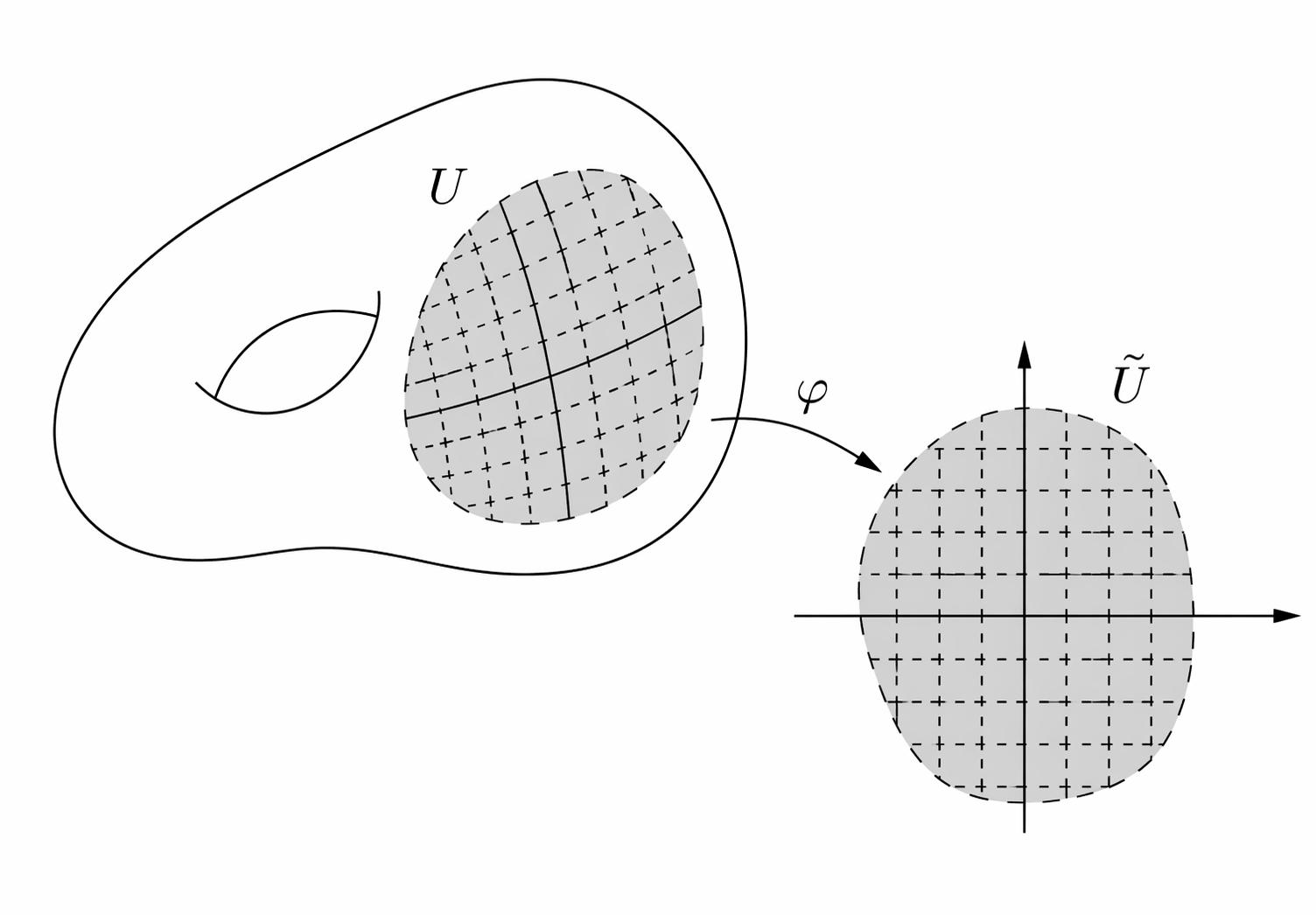
It excludes things like crosses, since the neighborhood of an intersection point can neither be mapped to an open subset of \(\mathbb{R}\) nor \(\mathbb{R}^2\) (a cross is not open in \(\mathbb{R}^2\)), and topological spaces that have a boundary (e.g. a disk), since neighborhood of points at the boundary would always map to non-open sets of \(\mathbb{R}^n\). This also excludes spaces like fractals and graphs.
What about “Haussdorf” and “second-countable”? Haussdorf means that distinct points have disjoint neighborhoods (it excludes for instance a line with two origins) and second-countable means that there exists a countable basis of open sets, such that every open set can be decomposed in this basis (it excludes for instance an uncountable number of copies of a line). Those are technical details which are important to avoid pathological cases and make many theorems work, but don’t linger over them too much. Simply think of a manifold as a continuous shape without boundaries or crossing points, like a sphere or a torus.
Finally, we say that a manifold is \(\bm{D}\)-dimensional if the neighborhood of every point can be mapped to an open set of \(\mathbb{R}^D\).
A nice property of manifolds is that they can be cellulated. There are many ways to define cellulations on a manifold. A simple way, which is the most relevant in the context of quantum error correction, is by using polytopes (the \(D\)-dimensional generalization of polygons). The cellulation of a manifold can then be defined as a set of polytopes, and a map (homeomorphism) from every polytope to the manifold, such that the manifold is fully covered and the polytopes only intersect at their faces. Here is an example of cellulation of 2D torus:
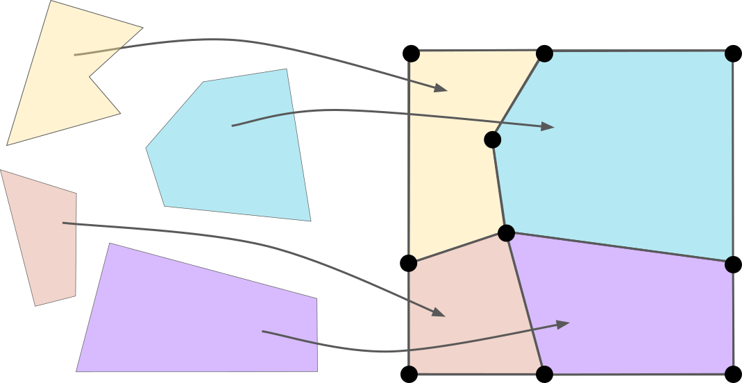
Note that I use here the same representation of the torus as when I defined the toric code: a square with top-bottom and left-right boundaries identified. This can be made rigorous topologically, by defining the manifold as the square \(S=[0,1]^2\) quotiented by an equivalence relation \(\sim\) such that top-bottom boundaries are equivalent, i.e. \((x,0) \sim (x,1)\) for all \(x \in [0,1]\), and left-right boundaries are equivalent, i.e. \((0,y) \sim (1,y)\) for all \(y \in [0,1]\). We discussed the notion of quotient before in the context of logical operators, defining the quotient of a group (the logicals) by a subgroup (the stabilizers). The idea for topological spaces is similar: the quotient \(\mathcal{M}=S/\sim\) of the topological space \(S\) (our square) by the equivalence relation \(\sim\) is formally defined as a space of sets (called cosets) such that each coset contained equivalent points. In our case, cosets corresponding to points in the bulk of our square are singleton, e.g. \(\{ (0.5, 0.2) \}\), while cosets corresponding to points at the boundaries contain either two elements, e.g. \(\{ (0,0.5), (1,0.5) \}\) or four for the corners, e.g. \(\{(0,0),(0,1),(1,0),(1,1)\}\). We can make this quotient a topological space by defining the neighborhood of points at the boundary to correspond to the union of neighborhoods on both sides, and then prove that it is actually a manifold, fulfilling all the properties of manifolds discussed above.
For any cellulation of a \(D\)-dimensional manifold, a \(\bm{k}\)-cell of this cellulation (for \(k \in \{ 0,\ldots,D \}\)) is the image of a \(k\)-dimensional face of one of the polytopes. For instance, \(0\)-cells are vertices of the cellulation, \(1\)-cells edges, \(2\)-cells, faces, etc.
As we will soon see, one can learn invariant properties of the manifold by using only the combinatorial description of any cellulation of the manifold. By combinatorial description, I simply mean how our polytopes are connected to each other, rather than their exact shape. And a nice way to formalize this notion is through the concept of chain complex.
Chain complexes
There is a famous adage in maths communities saying that all mathematics can be reduced to either linear algebra or combinatorics. Chain complexes reduce the study of topological manifolds to both.
Let’s consider a cellulation of a \(D\)-dimensional manifold.
Homology and cohomology
Conclusion
Problem with a fix Euclidean manifold
-
To be more precise, I should write \((H_X^{(\ell)},H_Z^{(\ell)})\) to emphasize that we are dealing with a family of codes indexed by an integer \(\ell\), and not just a single code (e.g. \(\ell\) would be the lattice size for the surface code). The parameters of the code family could then also be written \([[n_\ell,k_\ell,d_\ell]]\). I omit the index here and in the rest of the post to avoid overloading the notations, as it should be clear from context when there is an implicit dependency on some integers \(\ell\). ↩︎