An interactive introduction to the surface code
Last July, the quantum team at Google released a milestone paper, in which they show the first experimental demonstration of quantum error correction below threshold. What this means is that their experiment reached noise levels that are low enough such that by increasing the size of their code, they progressively reduced the number of errors in the encoded qubit. And how did they achieve such a milestone? You guessed it, by using the surface code to protect their qubits! The reasons they chose this code are plentiful: it can be laid down on a 2D lattice, it has a very high threshold compared to other codes, it doesn’t require too many qubits in its smallest instances, etc. And Google is far from the only company considering the surface code (or some of its variants) as part of their fault-tolerant architecture!
Apart from its experimental relevance, the surface code is also one of the most beautiful ideas of quantum computing, and if you ask me, of all physics. Inspired by the condensed matter concepts of topological order and anyonic particle, it was discovered by Alexei Kitaev in 1997, in a paper in which he also introduces the idea of topological quantum computing. And indeed, the surface code has deep connections to many areas of maths and physics. For instance, in condensed matter theory, the surface code (more often called toric code in this context1) is used as a prime example of topological phase of matter and is related to the more general family of spin liquids. While this post will be mainly concerned with the quantum error correction properties of the surface code, my friend Dominik Kufel wrote an excellent complementary post which describes the condensed matter perspective.
Finally, the surface code is the simplest example to illustrate the more general concept of topological quantum error-correction. While we will only consider surface codes defined on a 2D square lattice here, they can actually be generalized to the cellulation of any manifold in any dimension (including hyperbolic!). Concepts from algebraic topology (such as homology and cohomology groups, chain complexes, etc.) can then be used to understand and analyze those codes. While we will take a brief glance at topology here, I am planning to write a separate blog post fully dedicated to the maths behind topological quantum error-correction. The goal of this post is to gain a first intuitive understanding of the surface code.
You got it, I love the surface code, and I’m super excited to talk about it in this post! To do this code the honor it deserves, I’ve decided to make use of the interactive code visualizer I have been developing for some time with my collaborator Eric Huang. I’ve embedded it in this post2, and you will therefore be able to play with some of the lattices presented here (e.g. by inserting errors and stabilizers, visualizing decoding, etc.). I hope you’ll enjoy!
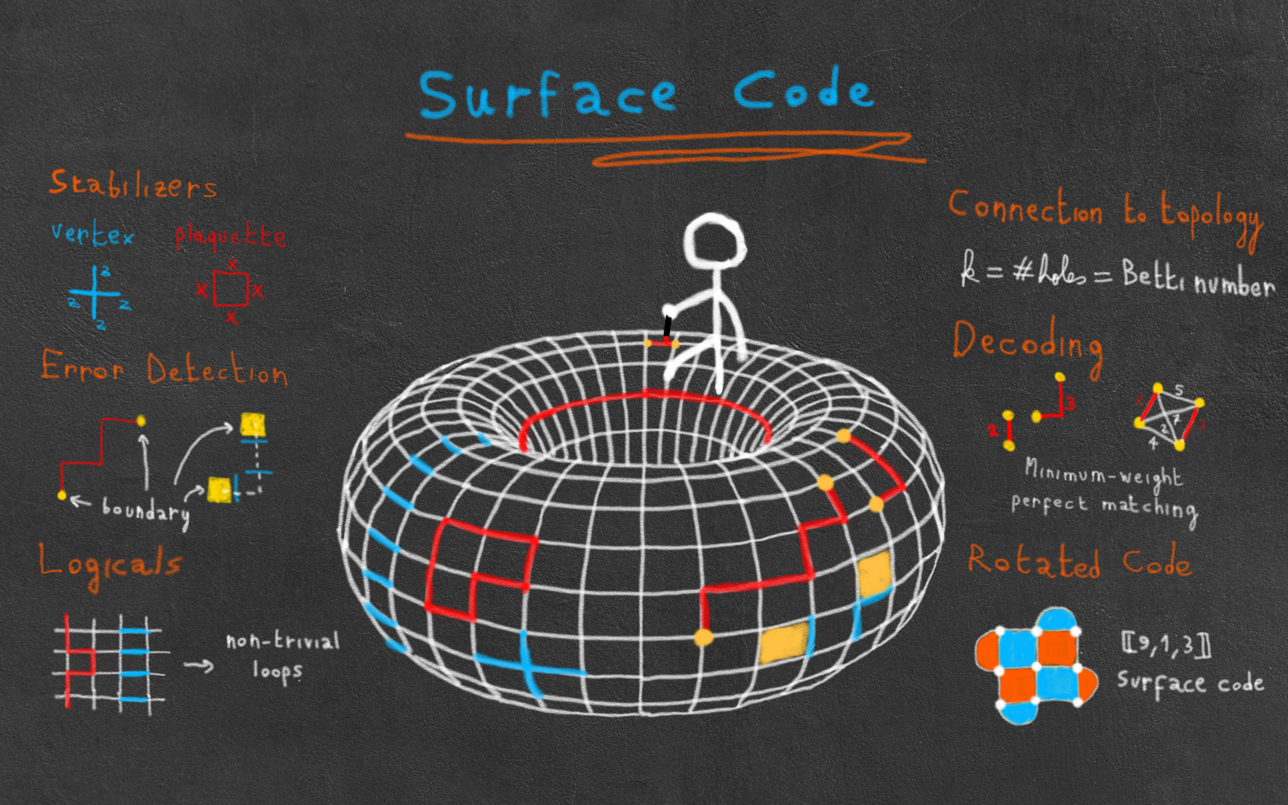
So here is the plan for today’s post. We will first look at the definition of the surface code on a torus by laying out its stabilizers, see how to detect errors, and delve into topology in order to understand the logical operators of the code. We will then study the decoding problem and see how it can be simplified to a matching problem on a graph. Next, we will introduce the planar code and the rotated code, variants of the surface code with more practical boundary conditions and a lower overhead. Finally, we will define the notion of error correction threshold and give its different values for the surface code.
This post assumes familiarity with the stabilizer formalism, so don’t hesitate to read my blog post series on the topic if you need a reminder.
Definition of the surface code
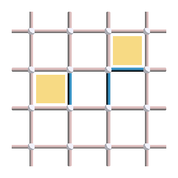
The surface code can be defined on a square grid of size \(L \times L\), where qubits sit on the edges, as shown here for \(L=4\):
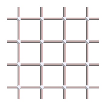
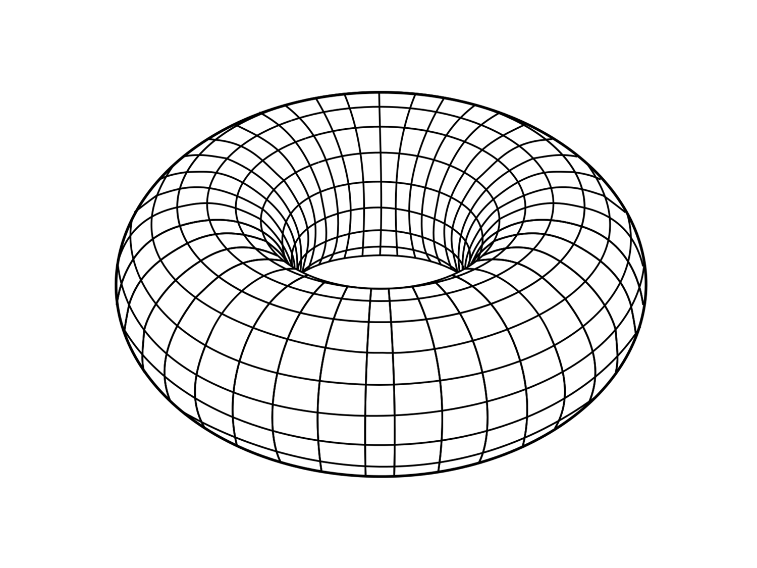
The code is easier to analyze at first when considering periodic boundary conditions. Therefore, in the picture above, we identify the left-most and right-most qubits, as well as the top-most and bottom-most qubits. The grid is therefore equivalent to a pac-man grid, or in topological terms, a torus. A torus as you might imagine it can be obtained from the grid by wrapping it around top to bottom (gluing the top and bottom edges together), making a cylinder, then left to right (gluing the left and right edges together) to finish the torus:
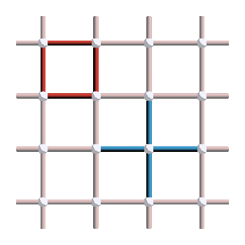
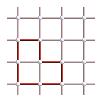
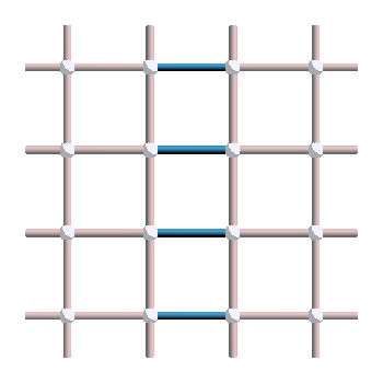
The next step is then to describe the stabilizers of the code. The surface code is indeed an example of stabilizer codes and can therefore be completely specified by its stabilizer group. In our case, we have two types of stabilizer generators: the vertex stabilizers, defined on every vertex of the lattice as a cross of four \(Z\) operators, and the plaquette stabilizers, defined on every face as a square of four \(X\) operators. Examples of vertex and plaquette stabilizers are shown below, where red means \(X\) and blue mean \(Z\).
To define a valid code, \(X\) and \(Z\) stabilizers must commute. Since they are Pauli operators, it means that they must always intersect on an even number of qubits. You can check that this is the case here: vertex and plaquette operators always intersect on either zero or two qubits.
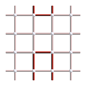
Since the stabilizer group is a group, it means that the product of stabilizers is also a stabilizer. Therefore, any product of plaquettes is also a stabilizer. Here is an example of product of three plaquettes:
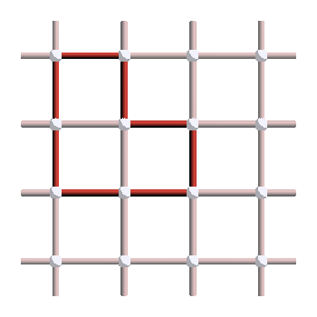
You can notice that this forms a loop! The reason is that when multiplying the plaquette operators, there are always two \(X\) operators applied on each qubit of the bulk, which cancel each other. This observation is true in general: all the \(X\) stabilizers are loops in the lattice! To convince yourself of that fact, try inserting plaquette stabilizers in the following panel:
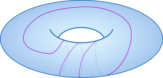
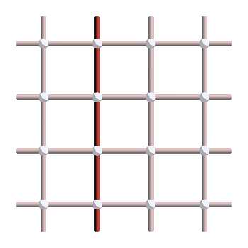
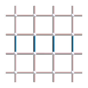
What about \(Z\) stabilizers? They also form loops… if we look at them the right way! Try to understand why by inserting vertex stabilizers in the following panel:
For instance, here is the product of three vertex operators:
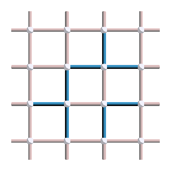
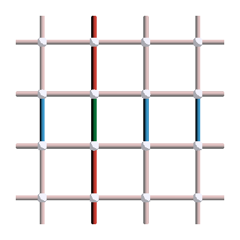
Can you see the loop? If no, this picture should make it clearer:
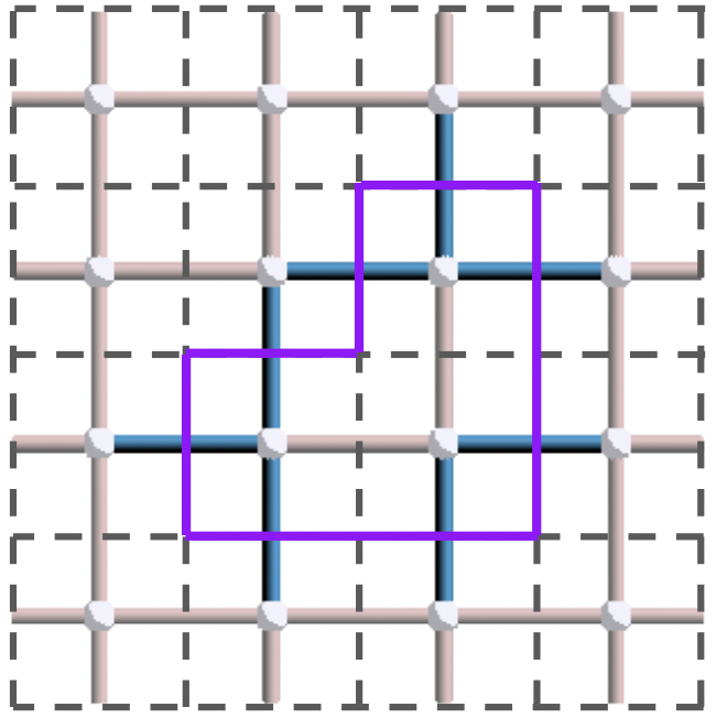
The trick was to draw an edge orthogonal to every blue edge (dashed purple lines on the figure). Formally, this corresponds to representing the operator in the so-called dual lattice, a lattice formed by rotating each edge by 90° (dashed grey lattice in the figure). In this lattice, vertex stabilizers have a square-like shape, similar to the plaquette stabilizers of the primal lattice. Therefore, all the properties we can derive for \(X\) stabilizers, errors and logicals can be directly translated to \(Z\) operators by simply considering the dual lattice, where \(Z\) operators behave exactly like \(X\) operators.
So we’ve seen that all the \(X\) and \(Z\) stabilizers are loops in the lattice. But is the converse true, that is, do all the loops define stabilizers? Try to think about this question, we will come back to it later.
Detecting errors
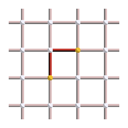
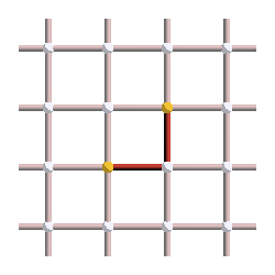
So what happens when errors start occurring on our code? Use the panel below to insert \(X\) and \(Z\) errors in the code:
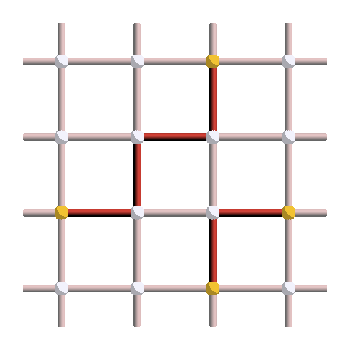
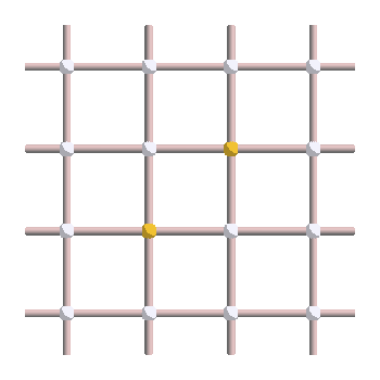
Vertices lighted up in yellow are the ones which anticommute with the error and are equal to \(-1\). They are part of the syndrome (set of measured stabilizer values) and are often called excitations or defects. Can you spot a pattern in the way excitations relates to errors? Let me help you. Start by removing all the errors. Then, draw a path of errors. Can you see what happens?
Excitations only appear at the boundary of error paths! Here is an example of pattern that should make that clear:
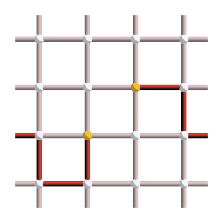
We can see that excitations are always created in pairs, and move through the lattice when increasing the size of the error string. What about \(Z\) errors? The same phenomenon occurs if errors paths are created by adding errors on parallel edges:
As expected, when seen in the dual lattice (i.e. when rotating each edge by 90°), those \(Z\) paths correspond to regular strings of errors.
The fact that excitations live at the boundary of error paths also means that when a path forms a loop, the excitations disappear. In other words, loops always commute with all the stabilizers. And what is an operator that commutes with all the stabilizers? A logical operator!
Logical operators, loops and topology
A logical operator can either be trivial, in which case it is a stabilizer, or non-trivial, in which case it performs an \(X\), \(Y\) or \(Z\) logical operation on any of the \(k\) qubits encoded in the code. For the surface code, the distinction between all those different operators depends on the types of loop they form. And this where the connection with topology really begins. Let’s first study the structure of loops on a general smooth manifold, before applying it to the surface code.
Loops on a smooth manifold
Let’s consider a smooth manifold \(\mathcal{M}\) (e.g. a torus). We say that two loops on \(\mathcal{M}\) are equivalent if there exists a smooth deformation of one loop to the other, meaning that we can smoothly move the first loop to the other loop without cutting it3. For instance, the following four loops (green) on the torus are equivalent:
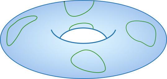
Moreover, we say that a loop is contractible, or trivial, if it is equivalent to a point, that is, we can smoothly reduce it until it becomes a single point. All the loops in the figure above are examples of contractible loops on the torus. So what do non-contractible loops look like? Here are examples of non-contractible loops:
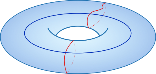
One loop (blue) goes around the middle hole, while two loops (red) goes around the hole formed by the inside of the donut. Note that those types of loop (red and blue) are not equivalent to each other, and cannot be deformed to obtain any of the green loops of the first figure neither.
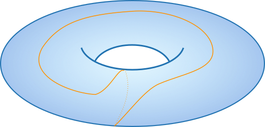
As always when we define a notion of equivalence, it can be interesting to look at all the different equivalence classes that they lead to. As a reminder, an equivalence class, or coset, is a set containing all the objects equivalent to a reference object. So let’s enumerate all the equivalence classes of loops on the torus. First, we have the contractible loops. They are all equivalent, since each of them can be reduced to a point, and two points can always be smoothly moved to each other. So that’s our first equivalent class, that we can call the trivial class. Then, we have the red and blue loops of the figure above: one that goes around the middle hole and the other that goes around the hole formed by the inside of the donut. That’s two other equivalent classes. Note that a pair of loops is also technically a loop itself, so taking the red and blue loops together forms its own loop, which is not equivalent to either one of them separately. This “double loop” can also be understood as (and is equivalent to) a single loop that goes around both holes, like the orange line in the picture below:
So that’s a fourth equivalence class. Do we have more?
Yes! Loops going around a hole twice are not equivalent to loops going around the hole once. Therefore, for each \(k \in \mathbb{N}\), we have a new class of loops going around one of the holes \(k\) times. Since in general loops are given a direction, we can also consider loops going around each hole in the opposite direction and take \(k \in \mathbb{Z}\). Overall, there are infinitely-many equivalence classes which can be labeled by two integers \((k_1,k_2) \in \mathbb{Z}^2\), where each integer indicates how many times the loops go around the corresponding hole. In this notation, the trivial class corresponds to \((0,0)\), the blue and red non-trivial loops correspond to \((0,1)\) and \((1,0)\), and the orange loop corresponds to \((1,1)\).
Loops on the surface code
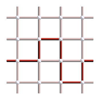
How can we apply what we have learned to the surface code? Compared to general smooth manifolds, the surface code has a more discrete structure, and the notion of smoothly deforming a loop does not directly apply here. We need a slightly different notion of equivalence4. We say that two loops \(\ell_1,\ell_2\) on the surface code are equivalent if there exists a stabilizer \(S \in \mathcal{S}\) such that \(\ell_1 = S \ell_2\). For instance, if we consider \(X\) errors and \(X\) stabilizers, two loops of errors are equivalent if we can apply a series of plaquettes to go from one to the other. As an exercise, show that the following two loops are equivalent, by finding some plaquettes that move one loop to the other:
Note that this notion of equivalence is exactly the same as the notion of logical equivalence defined in Part II of the stabilizer formalism series: applying a stabilizer to a logical gives another representation of the same logical. So operationally, two loops are equivalent if they correspond to the same logical operator. Therefore, by looking at all the equivalence classes of loops, we will be able to classify the different logical operators of the code.
Now, we say that a loop is contractible, or trivial, if it is equivalent to the empty loop (no error). In other words, a loop is trivial if it is a stabilizer. In the case of \(X\) errors, a trivial loop corresponds to the boundary of a set of faces (the plaquettes that form the stabilizer).
We are now ready to answer our main question. What are the non-trivial loops of the surface code, or in other words, the non-trivial logical operators? For \(X\) errors, they look like this:
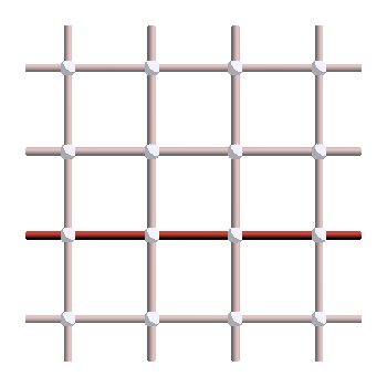
And since applying plaquette stabilizers does not change the logical operator, the following strings give other valid representatives of the same logicals:
As in the smooth case, what matters is that the non-trivial loops go around the torus. Indeed, you will not be able to write those operators as products of plaquette stabilizers. Operationally, each of those two loops (the “horizontal” and the “vertical” ones) correspond to applying a logical \(X\) operator to the code, and since they are not equivalent, they are applying it to different logical qubits. Therefore, we have at least two logical qubits, one for the horizontal loop and one for the vertical loop. Do we have more?
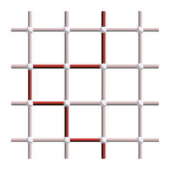
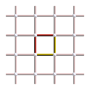
This time, we only have four different cosets of loops. Indeed, contrary to the smooth case, looping around the lattice twice always gives a trivial loop. This can be seen in two ways. The first way consists in observing that a loop going around the lattice twice is always equivalent to two disjoint loops (this was also true in the smooth case).
The next step is then to show that such a two-loop pattern is always a stabilizer. For instance, try to find the plaquette stabilizers that give rise to the two loops on the right picture:
The second way to see this is to remember that a loop applies a logical operator \(P\), and applying this logical operator twice gives \(P^2=I\). It means that any double loop lives in the identity coset, and is therefore a stabilizer.
Thus, our equivalence classes for \(X\) errors can be labeled by two bits \((k_1,k_2) \in \mathbb{Z}_2 \times \mathbb{Z}_2\). The corresponding logical operators are \(I\), \(X_1\), \(X_2\) and \(X_1 X_2\). The fact that our sets are \(\mathbb{Z}_2\) instead of \(\mathbb{Z}\) can also be interpreted as a consequence of the fact that we have qubits. For qudits, the generalization of Pauli operators obey \(P^d=I\), and \(\mathbb{Z}_2\) is replaced by \(\mathbb{Z}_d\). For error-correcting codes on continuous-variable systems (roughly, qudits with \(d=\infty\)), we recover \(\mathbb{Z}\) as our space of equivalence classes5.
Let’s summarize what we have learned. Loops of the surface code define logical operators. There are four non-equivalent types of loops: the trivial ones (stabilizers), the horizontal ones (\(X_1\) operator), the vertical ones (\(X_2\) operator), and those two at the same time (\(X_1 X_2\) operator). Therefore, the surface code encodes \(k=2\) logical qubits.
Note that in general, the surface code can be defined on any smooth manifold \(\mathcal{M}\) by discretizing it. The number of logical qubits of the code is then directly connected to the topological properties of the manifold, and in particular, to the number of holes, or in more technical terms, the first Betti number of the manifold. For instance, for the torus, the fact that \(k=2\) is a consequence of the presence of two holes.
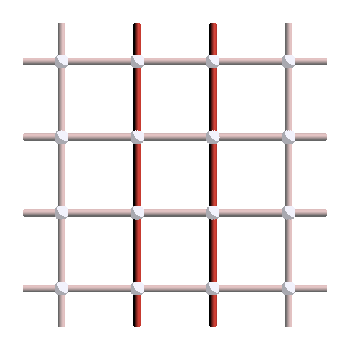
So far, we have mainly discussed loops of \(X\) errors, but what about \(Z\) errors? As expected, the \(Z_1\) and \(Z_2\) logicals correspond to loops going around the torus when considered in the dual lattice:
On the left is the \(Z_1\) logical (which anticommute with \(X_1\)) and on the right is the \(Z_2\) logical (which anticommute with \(X_2\)). Those anticommutation relation between \(X_1\) and \(Z_1\) can be seen in this picture:
Indeed, we can see that the \(X_1\) and \(Z_1\) logicals intersect on exactly one qubit (green), meaning that they anticommute. This property is independent on the specific logical representatives you choose: a “horizontal” \(X\) loop will always intersect with a “vertical” \(Z\) loop on a single qubit.
You now have all you need to determine the parameters of the surface code!
Decoding the surface code
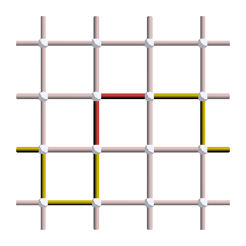
Let’s imagine that you observe the following syndrome, and want to find a good correction operator.
We know that excitations always appear in pairs, and correspond to the boundary of strings of errors. So the error must be a string that links those two excitations. However, the number of strings that could have given this syndrome is very large! Here are three examples of errors leading to the syndrome shown above:
Let’s suppose that the first pattern was our actual error, but we chose the middle pattern instead as our correction operator. This is what the final pattern, corresponding to the error (red) plus the correction operator (yellow), would look like:
And as you can see, this is a stabilizer! So applying this correction operator puts us back in the original state and the correction is a success. On the other hand, here is what would happen if we had applied the last correction operator instead:
As you can see, this is a logical operator! So this is an example of correction failure, where we have changed the logical state of our code when applying the correction.
What lessons can we draw from this example? The goal of the surface code decoding problem is to match the excitations such that the final operator is a stabilizer. Let’s try to formalize this a little. I described the general decoding problem for stabilizer codes in a previous post, but a short reminder is probably warranted.
Similarly to how logical operators can be partitioned into cosets, we can also enumerate equivalent classes for errors fitting a given syndrome. For instance, the first and middle patterns in our example above are part of the same equivalent class, as they can be related by a plaquette stabilizer. On the other hand, the last string belongs to a different class. The goal of decoding is to find a correction operator that belongs to the same coset as the actual error. Indeed, the product \(CE\) of the correction operator with the error is equal to a stabilizer if and only if there is a stabilizer \(S\) such that \(C=ES\), that is, if \(C\) and \(E\) belong to the same class. To solve this problem with the information we have, that is, only the syndrome and the error probabilities, the optimal decoding problem, also called maximum-likelihood decoding, can be formulated as finding the coset \(\bm{\bar{C}}\) with the highest probability:
\[\begin{aligned} \max_{\bm{\bar{C}}} P(\bm{\bar{C}}) \end{aligned}\]where \(P(\bm{\bar{C}})\) can be calculated as a sum over all the operators in the coset: \(P(\bm{\bar{C}}) = \sum_{\bm{C} \in \bm{\bar{C}}} P(\bm{C})\).
Solving this problem exactly is computationally very hard, as it requires calculating a sum over an exponential number of terms (in the size of the lattice). But for the surface code, it can be approximated very well using tensor network decoders, which have a complexity of \(O(n \chi^3)\) (up to some logarithmic factor), with \(n\) the number of qubits and \(\chi\) a parameter quantifying the degree of approximation of the decoder (corresponding to the bound dimension of the tensor network). The main downside of this decoder is that it generalizes poorly to the case of imperfect syndrome measurements. In this case, measurements need to be repeated in time, leading to a 3D decoding problem that tensor networks cannot solve efficiently at the moment.
As discussed in my stabilizer decoding post, the maximum-likelihood decoding problem can also be approximated by solving for the error with the highest probability, instead of the whole coset. Assuming i.i.d. noise, finding the error with the highest probability is equivalent to finding the smallest error that fits the syndrome. In the case of the surface code, this corresponds to matching the excitations with chains of minimum weight.
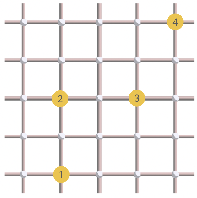
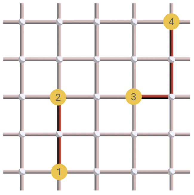
As it happens, this is completely equivalent to solving a famous graph problem, known as minimum-weight perfect matching! This problem can be expressed as matching all the vertices of a weighted graph (with an even number of vertices), such that the total weight is minimized. In our case, the graph is constructed as a complete graph with a vertex for each excitation. The weight of each edge between two vertices is then given by the Manhattan distance between the two corresponding excitations. For instance, let’s consider the following decoding problem:
The associated graph is then the following:
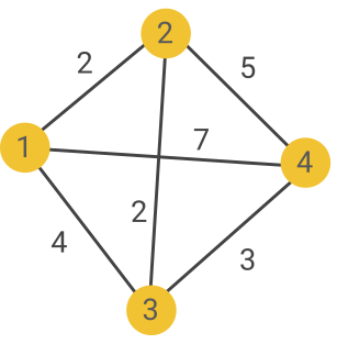
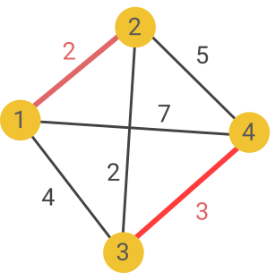
By enumerating all the possible matchings, you can quickly see that the one of minimum weight links vertices 1 and 2, and 3 and 4, with a total weight of 5:
From there, we can deduce our decoding solution:
It happens that minimum-weight perfect-matching can be solved in polynomial time using the Blossom algorithm, which has a worst-case complexity of \(O(n^3)\). While this complexity might seem quite high, a recent modification of the Blossom algorithm, proposed by Oscar Higgott and Craig Gidney, seems to have an average complexity of \(O(n)\). It also generalizes very well to the imperfect syndrome case, making it one of the best decoders out there in terms of trade-off between speed and performance (the performance will be reviewed when talking about thresholds in the last section of the post).
You can play with the matching decoder in the following visualization6:
There are many other surface code decoders out there with their own pros and cons, such as union-find, neural network-based decoders, belief propagation, etc. Describing them all in detail is out of scope for this blog post, but I hope to write a separate post one day dedicated to decoding. I also haven’t talked much about the decoding problem for imperfect syndrome, which I also leave for a separate blog post.
Let’s now answer a question that you might have been wondering this whole time: how the hell do we implement a toric lattice in practice? While it’s in principle possible to implement an actual torus experimentally (for example with cold atoms), it is impractical for many quantum computing architecture. Fortunately, there exists a purely planar version of the surface code, that we will discuss now!
Surface code with open boundaries
Consider the following version of the surface code, where vertex stabilizers on the top and bottom boundaries, and plaquette stabilizers on the left and right boundaries, are now supported on three qubits instead of four:
We call the top and bottom boundaries smooth boundaries, and the left and right boundaries rough boundaries. Feel free to play with this lattice and try to figure out what the main differences are, compared to the toric code. In particular, can you identify the logical operators of this code? How many equivalent classes, or logical qubits, can you spot?
The first difference to notice is that excitations can now be created at the boundary!
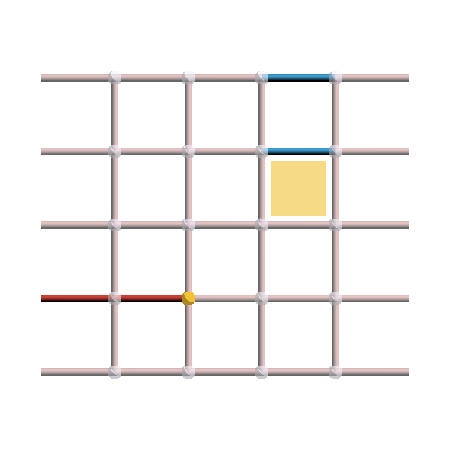
In this example, a vertex excitation is created on the rough boundary, and a plaquette excitation is created on the smooth boundary. You can see that excitations don’t have to come in pairs anymore! This poses a slight issue when decoding using minimum-weight perfect matching, but this can easily be overcome by adding some new boundary nodes to the matching graph.
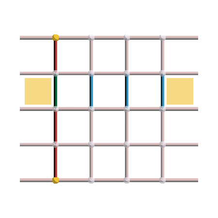
More importantly, we can observe that vertex excitations can only be created or annihilated at the rough boundaries, and plaquette excitations only at the smooth boundaries. This means that \(X\) logicals have to join the rough boundaries, and \(Z\) logicals have to join the smooth boundaries. This is illustrated in the following figure, where we can see that there is no “vertical” \(X\) logical or “horizontal” \(Z\) logical.
Therefore, there are only two equivalence classes of logicals for each error type: the strings that join opposite boundaries, and the trivial loops. As a consequence, this non-periodic version of the surface code, also called planar code, only encodes a single qubit. It is a \([[2L^2 - 2L + 1, 1, L]]\)-code. While we have lost one qubit compared to the toric version, the fact that it can be laid out on a 2D surface makes it much more practical.
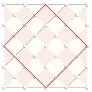
A more compact version: the rotated surface code
If you have started looking at the surface code literature, you might have noticed that people often use a different representation, which looks roughly like the following:
In this representation, qubits are on the vertices, and all the stabilizers are on the plaquette. Feel free to play with this lattice to understand what’s going on.
It happens that this lattice represents exactly the planar code that we saw before! Here are the two lattices on top of each other:
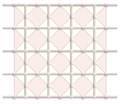
The idea is to turn every edge of the original representation into a vertex, each vertex into yellow face, and each face into a rose face. As a result, both vertices and plaquettes become rotated squares, and qubits become vertices. This representation is called the rectified lattice.
One advantage of this representation is that it allows you to come up with a different, more compact, version of the surface code. The idea is to take to following central piece of the rectified lattice:
We then rotate it and add a few boundary stabilizers. This gives the following code, called the rotated surface code:
As always, feel free to familiarize yourself with this new code by playing with it on the visualization. You should be able to see that it also encodes a single logical qubit, and has a distance of \(L\). However, this time, the number of physical qubits is exactly \(L^2\). The rotated surface code is therefore a \([[L^2, 1, L]]\)-code, which is a factor two improvement in the overhead compared to the original surface code. This version of the surface code is therefore the preferred one to realize experimentally. For instance, its two smallest instances, the \([[9,1,3]]\) code and the \([[16,1,4]]\) code are the ones recently realized by the Google lab.
When considering a code family such as the surface code, the \([[n,k,d]]\) parameters only give part of the story. Another very important characteristics of a code family is its set of thresholds.
Thresholds of the surface code
The threshold of a code family for a given noise model and decoder is the maximal physical error rate \(p_{th}\) such that for all \(p < p_{th}\), increasing the code size decreases the logical error rate. The threshold is typically calculated numerically using plots that look like the following:
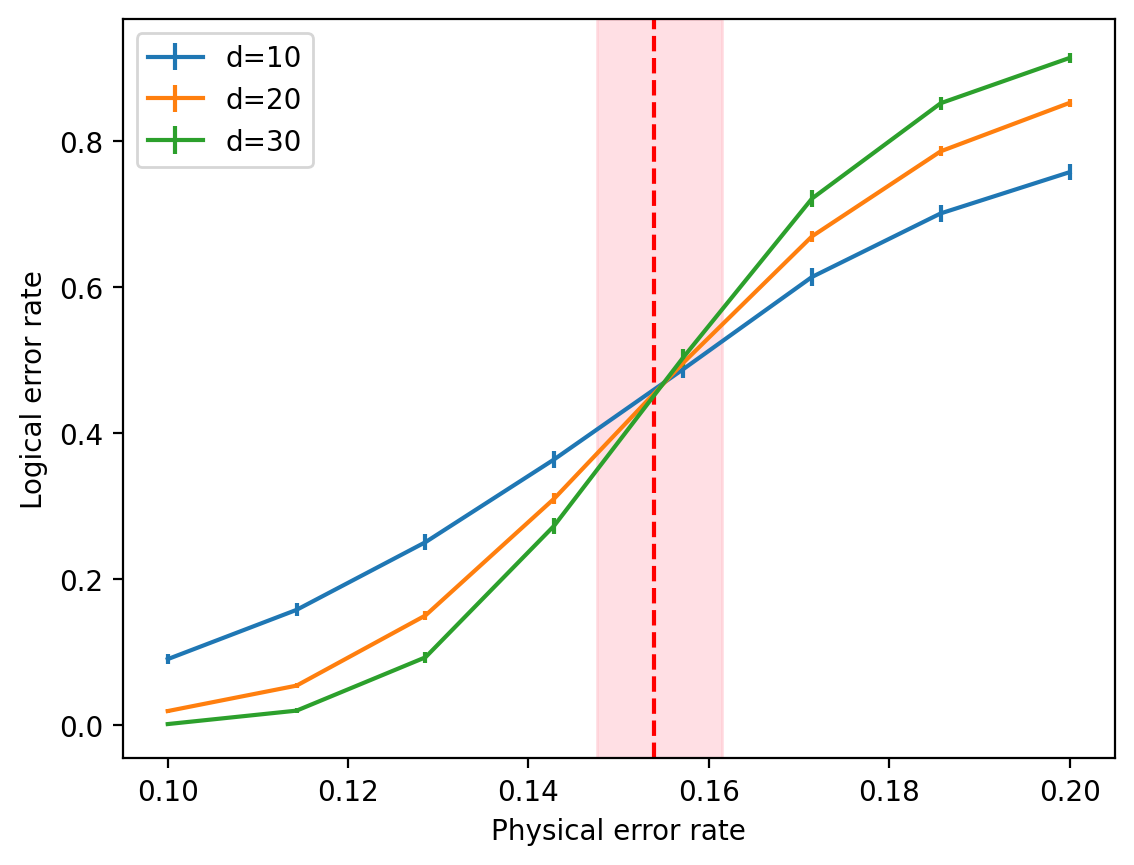
To make this figure, codes with distance \(10,20,30\) are simulated under noise channel with varying physical error rate. Errors are then decoded, and logical errors are enumerated. We can see that above \(p_{th} \approx 15.5\%\), increasing the code distance increases the logical error rate, while below \(p_{th}\), the logical error rate decreases with the code distance.
So what is the threshold of the surface code? First of all, very importantly, there isn’t a single threshold for the surface code: it highly depends on which noise channel and which decoder we are using. Let’s start by discussing noise models.
We often make the distinction between three types of noise models:
- The code-capacity model, in which errors can occur on all the physical qubits of the code, but measurements are assumed to be perfect.
- The phenomenological noise model, in which each stabilizer measurement can also fail with a fixed probability.
- The circuit-level noise model, in which the circuits to prepare the code and extract the syndrome are considered, and errors are assumed to occur with a certain probability after each physical gate.
The code-capacity threshold is the easiest to estimate, both in terms of implementation time and computational time, and allows to get a rough idea of the performance of a given code or decoder. The phenomenological threshold gets us closer to the true threshold value and can be useful when comparing decoders that deal with measurement errors in interesting ways (such as single-shot decoders). Finally, circuit-level thresholds are the most realistic ones and approximate the most accurately the actual noise level that experimentalists need to reach to make error correction work with a given code. While circuit-level thresholds have been considered very hard to estimate for a long time, mainly due to the lack of very fast noisy Clifford circuit simulators, recent tools such as Stim have made those simulations much less cumbersome.
For each of those three models, we also need to specify the distribution of \(X\), \(Y\) and \(Z\) errors7. There are two very common choices here. The first is the depolarizing noise model, in which those three Paulis are assumed to occur with the same probability. Since \(Y\) is made of \(X\) and \(Z\), it means that \(P(Y)=P(X,Z) \neq P(X)P(Z)\), or in other words, \(X\) and \(Z\) are correlated. Another noise model is the independent \(X/Z\) model, in which \(X\) and \(Z\) are independent and occur with the same probability. The probability of getting \(Y\) errors is fixed as \(P(Y)=P(X)P(Z)=P(X)^2\) and is therefore lower than for depolarizing noise.
Regarding the decoders, we will consider two of them here for simplicity: the maximum-likelihood decoder, and the matching decoder. As it happens, the code-capacity threshold for the maximum likelihood decoder corresponds exactly to the phase transition of a certain statistical mechanics model. This stat mech mapping was established in Dennis et al. (a classic of the quantum error correction literature) in 2002. For the surface code subjected to independent \(X/Z\) errors, the equivalent stat mech model is the random-bond Ising model, whose phase transition had just been calculated at that time. They were therefore able to give this first surface code threshold without doing any simulation themselves!
We are now ready to give the actual threshold values for the surface code! Here is a table with the code-capacity thresholds of the different noise models and decoder discussed previously:
| Maximum-likelihood | Matching | |
| Depolarizing noise | 18.9% | 15.5% |
| Independent noise | 10.9% | 10.5% |
Table 1: Code-capacity thresholds of the surface code
For phenomenological and circuit-level noise, I am only aware of some matching decoder thresholds under depolarizing noise. For phenomenological noise, we have a threshold of about \(3\%\). For circuit-level noise, the threshold goes down to about \(1\%\), which is often the cited value for “the threshold of the surface code”.
Conclusion
In this post, we have defined the surface code and its different variants (toric, planar, rotated) and tried to understand its most important properties visually. We have seen that it encodes one or two logical qubits depending on the boundary conditions, and has a distance scaling as \(\sqrt{N}\). Stabilizers can be thought as trivial (or contractible) loops on the underlying manifold, while the logical \(X\) and \(Z\) operators are the non-trivial loops going around the torus or joining the boundaries, drawing a connection between topology and codes. We have also studied the decoding problem for the surface code and how minimum-weight perfect matching can be used for this purpose. Finally, I have introduced the notion of error-correction threshold and given its value for different decoders and noise models.
The surface code is by far one of the most studied codes of the quantum error-correction literature and there is a lot more to say about it! I haven’t told you how to deal with measurement errors, how to prepare the code and measure the syndrome using quantum circuits, how to run logical gates on it, how to generalize it to different lattices and dimensions, how to make precise the connection with topology, etc. The surface code is also a stepping stone to understand more complicated codes, from the color code (the second most famous family of 2D codes) to hypergraph product codes and all the way to good LDPC codes. Now that you are equipped with the stabilizer formalism and have a good grasp of the surface code, the tree of possible learning trajectories has suddenly acquired many branches, and I hope to cover as many of those in subsequent blog posts!
In the meantime, one direct follow-up from this post is Dominik Kufel’s post on the condensed matter aspects of the toric code, where you will learn about the connection between codes and Hamiltonians, why excitations are called excitations and can be thought of as quasi-particles called anyons, what the state of the surface code looks like and how it provides an example of topological phase of matter. This connection is crucial to learn for any practicing quantum error-correcter, as it is used extensively in the literature and allows to understand many computational aspects of the surface code (how to make gates by braiding anyons, why the circuit to prepare the surface code has polynomial size, etc.). So go read his post!
Solution of the exercise
-
I tend to use the names surface code and toric code interchangeably. Some people use surface code to talk about the open-boundary version and toric code to talk about the periodic-boundary one, but this is not a universal convention, and the name planar code is also often used to talk about the open-boundary version. ↩︎
-
The final version of this embedding is just a few lines of Javascript, which use gui.quantumcodes.io as an API. So if you would like to embed some codes (both 2D and 3D) in your website, feel free to contact me, and I’ll give you the instructions to do it (I might add an official tutorial in the PanQEC documentation later). ↩︎
-
For the interested reader, the rigorous definition is that two loops are equivalent if there exists a homotopy between them. More precisely, we can define a loop as a continuous map \(\ell: S^1 \rightarrow \mathcal{M}\) (an embedding of the circle onto the manifold). A homotopy between two loops \(\ell_1, \ell_2\) is then a continuous function \(L:S^1 \times [0,1] \rightarrow \mathcal{M}\) such that \(L(\cdot, 0)=\ell_1\) and \(L(\cdot, 1)=\ell_2\). In other words, each \(L(\cdot, t)\) for \(t \in [0,1]\) defines a different loop on the path from \(\ell_1\) to \(\ell_2\). The equivalence relation defined here is called homotopy equivalence, and is one of the most important notions of equivalence in topology. ↩︎
-
This other notion of equivalence is called homological equivalence. Technically, two loops are homologically-equivalent if they can be seen as the boundary of a higher-dimensional object (in our case, the boundary of some plaquettes). In particular, trivial loops are the ones that are themselves boundaries of some objects (they are equivalent to the zero loop) and non-trivial loops are the ones that cannot be seen as boundaries. While the notion of homotopy is more powerful in general (it gives more information about a topological manifold), homology classes are usually simpler to calculate and are the right topological invariants for many practical applications. I will try to dedicate a post to the notion homology and its applications in quantum error correction. ↩︎
-
Rotor codes are example of such continuous-variable codes. ↩︎
-
The backend is using PyMatching, Oscar Higgott’s fast implementation of minimum-weight perfect matching. ↩︎
-
We assume here that we have a Pauli error model. The reasons for this choice are actually quite technical, and I hope to write a post about it one day. In the meantime, you can have a look at Section 10.3 of Nielsen & Chuang to get an idea of the argument. ↩︎