The topology of topological QEC I — Manifolds and complexes
To continue our journey into quantum error correction, it is time to dive deeper into the theoretical foundations of the field. When learning about the surface code, you might have wondered: what exactly makes it work? Would it work as well on lattices other than the square lattice? On manifolds other than the torus? In higher dimensions?
As it happens, the field of algebraic topology provides exactly the right tools to answer these questions. By understanding its basics, we can construct and study generalized surface codes and many other families of topological codes, such as color codes and fracton codes1. Furthermore, a generalization of algebraic topology, homological algebra, allows us to go beyond topological codes and serves as the foundation for most quantum LDPC code constructions and logical gate designs. The definitions and fundamental theorems from these two fields are therefore used all over the QEC literature, and studying them is well worth your time if you want to understand most modern fault-tolerant architecture constructions.
In this three-post series, we will explore the basics of algebraic topology with a quantum error correction lens. This first post focuses on constructions: you will learn about topological spaces, manifolds, cellulations, and chain complexes, and see how they can be used to build generalized surface codes. The second and third posts focus on properties, introducing homology and cohomology groups and explaining how they relate to the main properties of quantum codes.
As always, the main focus of this blog is on building intuition and visual understanding, and I therefore gloss over many technical details. However, if you are craving more details after reading these posts, I recommend consulting either Chapter 3 of my thesis or Chapter 2 of Niko Breuckmann’s thesis, where all the definitions and theorems are presented more formally.
Motivation
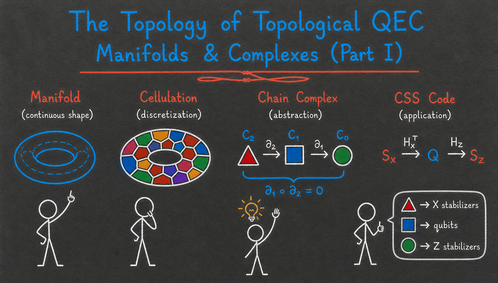
In Part III of the stabilizer trilogy, we saw that CSS codes can be described by two matrices, the parity-check matrices \(H_X\) and \(H_Z\), whose rows encode all the \(X\) and \(Z\) stabilizers of the code as binary vectors. For those two matrices to form a valid stabilizer code, they must obey the condition
\[\begin{aligned} H_X H_Z^T = 0 \end{aligned}\]which ensures that every \(X\) stabilizer must commute with every \(Z\) stabilizer. Furthermore, the parameters of the code can also be expressed using those matrices. For instance, the number of logical qubits \(k\) is exactly the dimension of the quotient space \(\ker(H_X)/\Im(H_Z^T)\). Why is that so? The kernel of \(H_X\) is the set of Pauli operators that commute with all the \(X\) stabilizers, that is, the (trivial and non-trivial) \(Z\) logical operators. Meanwhile, \(\Im(H_Z^T)\) corresponds to the set of \(Z\) stabilizers. The quotient therefore corresponds to equivalence classes of \(Z\) logicals up to stabilizers, with one class per logical qubit of the code. Another way to see it is through the identity
\[\begin{aligned} \dim \left( \ker(H_X) / \Im(H_Z^T) \right) = \dim(\ker(H_X)) - \dim(\Im(H_Z^T)) \end{aligned}\]Using the rank-nullity theorem, this becomes
\[\begin{aligned} \dim \left( \ker(H_X) / \Im(H_Z^T) \right) = n - \rank(H_X) - \rank(H_Z^T) \end{aligned}\]where \(\rank(H_X)=\rank(H_X^T)\) gives the number of independent \(X\) stabilizers, and \(\rank(H_Z^T)\) gives the number of independent \(Z\) stabilizers. This means that
\[\begin{aligned} \dim \left( \ker(H_X) / \Im(H_Z^T) \right) = n - m = k \end{aligned}\]with \(m\) the total number of independent stabilizers. We used the formula for the number of logical qubits that we saw in Part II of the stabilizer trilogy.
What about the distance? The \(X\) distance \(d_X\) is given by
\[\begin{aligned} d_X = \min_{L \in \ker(H_Z) \setminus \Im(H_X^T)} |L| \end{aligned}\]and similarly for the \(Z\) distance \(d_Z\). The total distance is then the minimum of \(d_X\) and \(d_Z\).
One last important property that can be read from the parity-check matrices is the locality of the code. It is not enough for a code to have good \([[n,k,d]]\) parameters, it must also have a good fault-tolerant implementation, that is, a set of circuits for syndrome extraction, state preparation, and logical gates, such that the error threshold is non-zero (i.e., there exists a non-zero physical error rate below which scaling the code and its circuits exponentially suppresses the logical error rate). One sufficient condition for a code family with growing distance to possess such a fault-tolerant implementation is for it to be a low-density parity-check (LDPC) code: each stabilizer acts on a constant number of qubits, and each qubit participates in a constant number of stabilizers. This was shown, for instance, in a classic 2013 paper by Daniel Gottesman. From the point of view of our matrices, a code family with parity-check matrices \((H_X,H_Z)\) is LDPC if both \(H_X\) and \(H_Z\) are sparse, that is, if the weight of their rows and columns remains constant as the code size increases2.
Where does this lead us? We can view CSS code design as the problem of finding families of matrix pairs \((H_X, H_Z)\), such that:
- \(H_X H_Z^T = 0\),
- \(H_X\) and \(H_Z\) are sparse,
- \(k\) is non-zero, and \(d\) is growing with the code size.
From a coding-theoretic perspective, satisfying these three constraints seems like a hard problem! In the classical setting, random LDPC codes are typically good, with both \(k\) and \(d\) scaling linearly with \(n\). However, naively trying to build two random matrices satisfying the orthogonality condition quickly runs into obstructions that prevent either sparsity or good parameters 3.
So we need a bit more structure if we want to satisfy all three constraints above. And this is where the magic begins: since the end of the 19th century, an entire field of mathematics has been devoted to studying exactly such matrices. I’m talking about the field of algebraic topology, and its extension, homological algebra.
Topological spaces, manifolds and cellulations
Algebraic topology can be described as the study of topological spaces and of quantities that remain invariant under continuous deformations of those spaces. This sentence contains a lot of important concepts, so let’s slowly decipher it. Topological spaces are sets equipped with a well-defined notion of neighborhood (satisfying certain axioms on their intersections and unions). They are very general objects, including familiar spaces such as \(\mathbb{R}^n\), spheres, tori, but also countable sets, graphs, and even fractals. The axioms of topological spaces are sufficient to generalize a number of notions from analysis, such as continuous functions and limits.
What about continuous deformations? Those are usually either homeomorphisms (continuous bijections with a continuous inverse) or homotopy equivalences (progressive continuous transformation of one space to another). This is where the famous saying that a mug and a donut are the same from a topological perspective comes from: they are homotopy equivalent.
Finally, the invariant quantities that are considered in algebraic topology are numbers or algebraic structures (groups, vector spaces, etc.) that allow us to classify topological spaces up to those deformations. For instance, to each topological space one can associate a sequence of groups, called homology groups, whose dimensions intuitively count the number of “\(k\)-dimensional holes” of the space. These quantities are invariant under homeomorphism and homotopy equivalence. We will see how these homology groups are constructed (and their interpretation in quantum error correction) very soon.
To understand how this works, let’s restrict our attention to a specific type of topological spaces, called topological manifolds (or simply manifolds for short). Formally, a manifold is a locally Euclidean Haussdorff second-countable topological space. ‘Locally Euclidean’ means that for every point, there is a neighborhood that is homeomorphic to an open subset of \(\mathbb{R}^n\) (for some \(n\)).
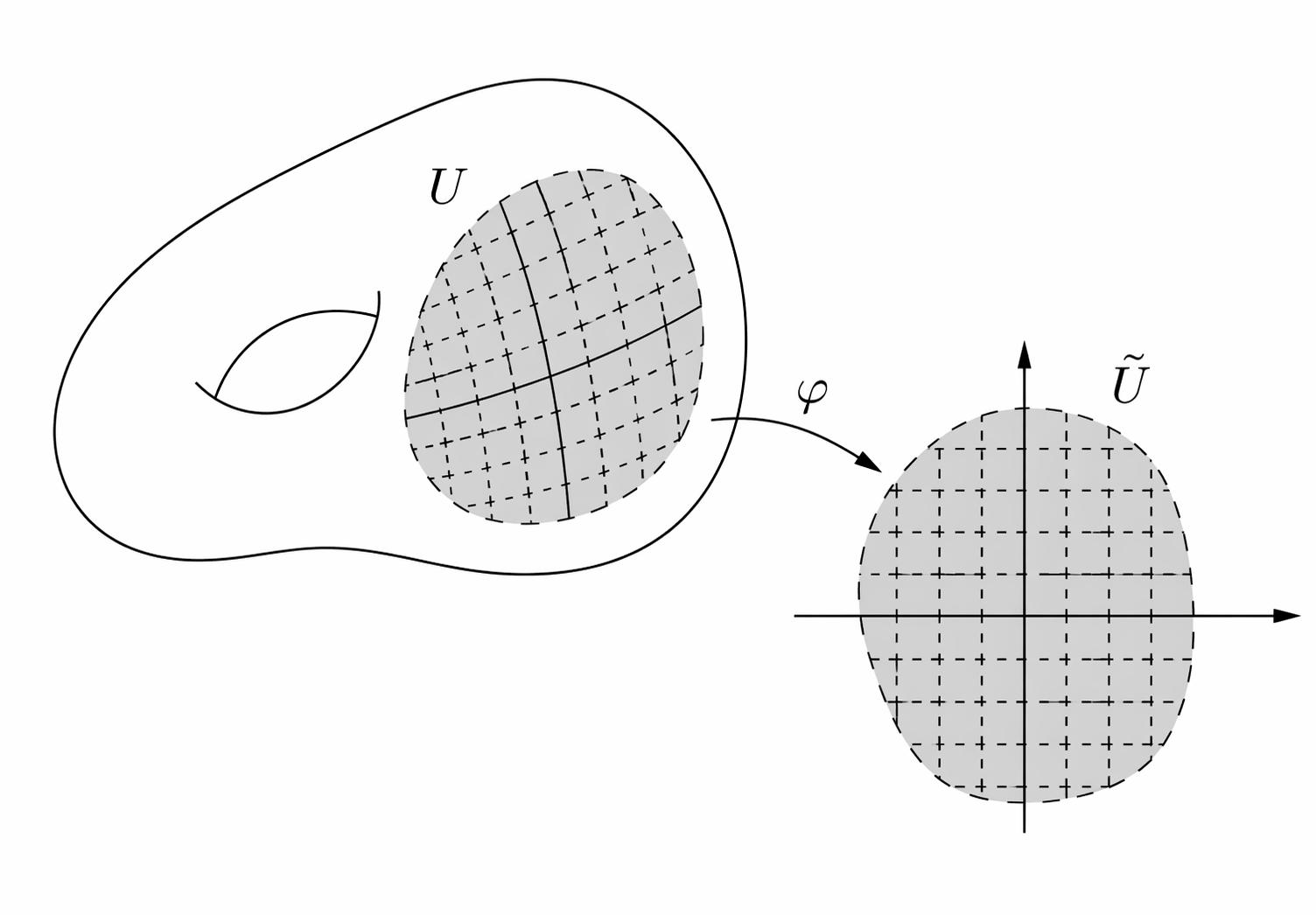
Homeomorphism from an open subset of a manifold to an open subset of \(\mathbb{R}^2\). Source: Daniel Irivine’s lecture notes
This definition excludes objects like countable sets, self-intersecting spaces like crosses or graphs (the neighborhood of an intersection point cannot be mapped to an open subset of any \(\mathbb{R}^n\)), or fractals. Strictly speaking, it also excludes topological spaces that have a boundary, such as disks, since the neighborhood of points at the boundary would not be open in \(\mathbb{R}^n\). However, the notion of manifold can be generalized to that of manifold with boundary, where neighborhood of boundary points are allowed to map to the half-spaces (\(\{x \in \mathbb{R}^n\, :\, x_0 \geq 0 \}\)). In what follows, we will use the term ‘manifold’ to include manifolds with boundary.
What about Haussdorff and second-countable? A space is Hausdorff if any two distinct points have disjoint neighborhoods (it excludes for instance a line with two origins) and it is second-countable if it admits a countable basis of open sets, such that every open set can be decomposed in this basis (it excludes for instance an uncountable disjoint union of lines). Those are technical details which are important to avoid pathological cases and make many theorems work, but we will not dwell on them too much. Simply think of a manifold as a continuous shape without crossing points, like a sphere, a torus or a disk.
Finally, we say that a manifold is \(\bm{D}\)-dimensional if the neighborhood of every point can be mapped to an open subset of \(\mathbb{R}^D\).
A nice property of manifolds is that they can be cellulated. There are many ways to define cellulations on a manifold. A simple approach, which is the most relevant in the context of quantum error correction, is to use polytopes (the \(D\)-dimensional generalization of polygons). The cellulation of a manifold is then given by a collection of polytopes, together with maps (homeomorphisms) from every polytope to the manifold, such that the manifold is fully covered and the polytopes intersect only along shared faces 4. Here is an example of cellulation of 2D torus:
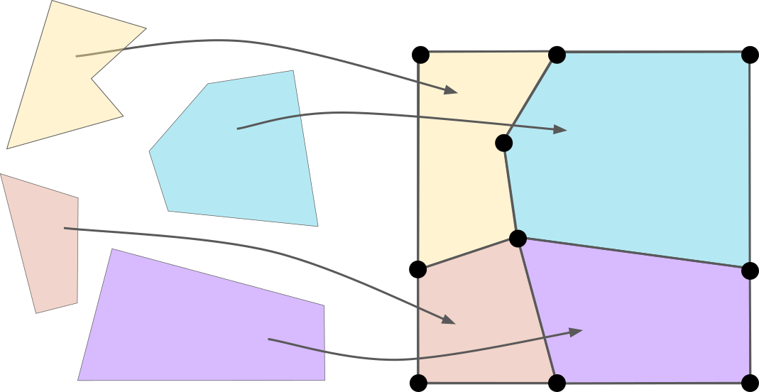
Here, I use the same representation of the torus as when I defined the toric code, namely a square with its top and bottom boundaries identified, as well as its left and right boundaries5.
For any cellulation of a \(D\)-dimensional manifold, a \(\bm{k}\)-cell of this cellulation (for \(k \in \{ 0,\ldots,D \}\)) is the image of a \(k\)-dimensional face of one of the polytopes. For instance, \(0\)-cells correspond to vertices, \(1\)-cells to edges, \(2\)-cells to faces, etc.
As we will soon see, many invariant properties of a manifold can be recovered purely from the combinatorial description of any of its cellulations. By combinatorial description, I simply mean how our polytopes are connected to each other, rather than their exact shapes. And a nice way to formalize this notion is through the notion of chain complex.
Chain complexes
There is a famous adage in mathematical communities saying that all mathematics can be reduced to either linear algebra or combinatorics. Chain complexes reduce the study of topological manifolds to both.
Let’s consider a cellulation of a \(D\)-dimensional manifold. For all \(i \in \{0,\ldots,D\}\), we denote by \(n_i\) the number of \(i\)-cells, and define the vector space
\[\begin{aligned} C_i = \mathbb{Z}_2^{n_i}. \end{aligned}\]We equip this vector space with a basis, where each basis element corresponds to a specific \(i\)-cell of the cellulation.
To make things concrete, consider the following cellulation of a square (a manifold with boundary, equivalent to the closed unit disk \(D^2\)), with \(n_0=4\) vertices, \(n_1=4\) edges, and \(n_2=1\) face.
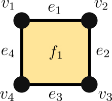
We then have
\[\begin{aligned} C_0 = \mathbb{Z}_2^{4},\;\; C_1 = \mathbb{Z}_2^{4},\;\; C_2 = \mathbb{Z}_2, \end{aligned}\]with the following bases:
\[\begin{aligned} C_0:& \;\; v_1 = \begin{pmatrix} 1 \\ 0 \\ 0 \\ 0 \end{pmatrix},\,\, v_2 = \begin{pmatrix} 0 \\ 1 \\ 0 \\ 0 \end{pmatrix},\,\, v_3 = \begin{pmatrix} 0 \\ 0 \\ 1 \\ 0 \end{pmatrix},\,\, v_4 = \begin{pmatrix} 0 \\ 0 \\ 0 \\ 1 \end{pmatrix} \\ C_1:& \;\; e_1 = \begin{pmatrix} 1 \\ 0 \\ 0 \\ 0 \end{pmatrix},\,\, e_2 = \begin{pmatrix} 0 \\ 1 \\ 0 \\ 0 \end{pmatrix},\,\, e_3 = \begin{pmatrix} 0 \\ 0 \\ 1 \\ 0 \end{pmatrix},\,\, e_4 = \begin{pmatrix} 0 \\ 0 \\ 0 \\ 1 \end{pmatrix} \\ C_2:& \;\; f_1=\begin{pmatrix} 1 \end{pmatrix} \\ \end{aligned}\]This allows us to represent any collection of \(i\)-cells as a vector of \(C_i\), by simply summing the corresponding basis vectors. For instance, the set consisting of the two top vertices of our square is represented by the vector
\[\begin{aligned} v = v_1 + v_2 = \begin{pmatrix} 1 \\ 1 \\ 0 \\ 0 \end{pmatrix}. \end{aligned}\]In other words, each entry equal to \(1\) in the vector indicates that the corresponding \(i\)-cell is included.
Next, we define some linear operators \(\partial_i:C_{i} \rightarrow C_{i-1}\), called boundary operators, which encode the incidence structure of the cellulation. More precisely, if an \(i\)-cell \(c \in C_i\) has boundary \(\{c_1,\ldots,c_\ell\}\), we define
\[\begin{aligned} \partial_i (c) = c_1 + \ldots + c_\ell. \end{aligned}\]In our example, \(\partial_2\) maps faces to edges, and \(\partial_1\) edges to vertices. We have
\[\begin{aligned} \partial_2 (f_1) = e_1 + e_2 + e_3 + e_4, \end{aligned}\]since the face \(f_1\) is connected to all four edges, and
\[\begin{aligned} \partial_1 (e_1) &= v_1 + v_2, \\ \partial_1 (e_2) &= v_2 + v_3, \\ \partial_1 (e_3) &= v_3 + v_4, \\ \partial_1 (e_4) &= v_4 + v_1 \end{aligned}\]since for instance \(e_1\) is incident to \(v_1\) and \(v_2\). We can also represent these operators as matrices:
\[\begin{aligned} \partial_2 &= \begin{pmatrix} 1 \\ 1 \\ 1 \\ 1 \end{pmatrix} \\ \partial_1 &= \begin{pmatrix} 1 & 0 & 0 & 1 \\ 1 & 1 & 0 & 0 \\ 0 & 1 & 1 & 0 \\ 0 & 0 & 1 & 1 \\ \end{pmatrix} \\ \end{aligned}\]From \(\partial_1\), we can read that \(e_1\) (first column) is incident to \(v_1\) and \(v_2\) (first and second rows), that \(e_2\) is incident to \(v_2\) and \(v_3\), and so on.
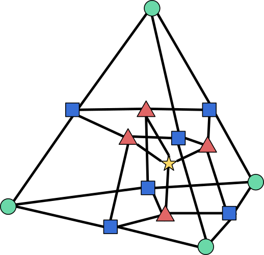
Alternatively, boundary operators can be viewed as biadjacency matrices of certain bipartite graphs. For any cellulation, we can indeed construct a \((D+1)\)-partite graph with one node for each \(i\)-cell, and an edge between an \(i\)-cell and an \((i-1)\)-cell whenever the latter lies in the boundary of the former. For instance, here is the graph associated with our cellulation of the square:
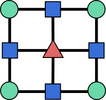
where circles represent \(0\)-cells, squares represent \(1\)-cells, and triangles represent \(2\)-cells. The boundary operator \(\partial_1\) is then the biadjacency matrix of the bipartite graph between circles and squares, while \(\partial_2\) is the biadjacency matrix of the bipartite graph between squares and triangles. Recall that the biadjacency matrix of a bipartite graph with node sets \(U\) and \(V\) is the matrix whose rows are indexed by nodes of \(U\), columns indexed by nodes of \(V\), and entries equal to \(1\) if there is an edge between the corresponding nodes, and \(0\) otherwise. This graph is sometimes called the Hasse diagram of the cellulation.
An important property of cellulations is that the boundary operators satisfy the following condition for any \(i \in \{0,\ldots,D-1\}\)6:
\[\begin{aligned} \partial_i \circ \partial_{i+1} = 0. \end{aligned}\]Intuitively, this reflects the fact that the boundary of a boundary is empty. For instance, in our example, we have
\[\begin{aligned} \partial_1 \partial_2 (f_1) &= \partial_1 (e_1 + e_2 + e_3 + e_4) \\ &= (v_1 + v_2) + (v_2 + v_3) + (v_3 + v_4) + (v_4 + v_1) \\ &= 0 \end{aligned}\]since each \(v_i\) appears twice in the sum, and we are working over \(\mathbb{Z}_2\).
We are now finally ready to introduce the notion of chain complex. A length-\(\bm{D}\) chain complex is a sequence of vector spaces \(C_0, \ldots, C_D\), along with linear operators \(\partial_i:C_i \rightarrow C_{i-1}\) satisfying the chain complex condition \(\partial_i \circ \partial_{i+1} = 0\) for all \(i \in \{0,\ldots,D-1\}\). We can represent a chain complex as a diagram:
\[\begin{aligned} C_D \xrightarrow{\partial_D} C_{D-1} \xrightarrow{\partial_{D-1}} \cdots \xrightarrow{\partial_2} C_1 \xrightarrow{\partial_1} C_0. \end{aligned}\]When the chain complex is constructed from a cellulation of a manifold, we call it a cell complex. However, the notion of chain complex is more general, and does not require any underlying manifold cellulation. It can be seen as a \((D+1)\)-partite graph with nodes of types \(0,\ldots,D\), edges only between successive types, and the constraint that the neighborhood of any node of type \(i\) must have even intersection with the neighborhood of every node of type \(i+2\), for all \(i \in \{0,\ldots,D-2\}\). For instance, you can check that the following graph defines a valid chain complex
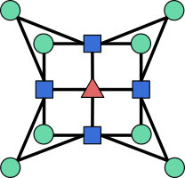
even though the square nodes cannot be interpreted as \(1\)-cells (edges) of a cellulation, since they are connected to four \(0\)-cells (vertices).
Back to QEC
You can probably already see where this is going. For any CSS code with \(n\) qubits, \(m_X\) \(X\) stabilizers, \(m_Z\) \(Z\) stabilizers, and parity-check matrices \(H_X\) and \(H_Z\), the condition \(H_Z H_X^T = 0\) implies that the following diagram defines a valid chain complex:
\[\begin{aligned} \mathcal{S}_X \xrightarrow{H_X^T} \mathcal{Q} \xrightarrow{H_Z} \mathcal{S}_Z, \end{aligned}\]where \(\mathcal{S}_X = \mathbb{Z}_2^{m_X}\), \(\mathcal{Q} = \mathbb{Z}_2^n\), and \(\mathcal{S}_Z = \mathbb{Z}_2^{m_Z}\). Conversely, any length-2 chain complex
\[\begin{aligned} C_2 \xrightarrow{\partial_2} C_1 \xrightarrow{\partial_1} C_0 \end{aligned}\]defines a valid CSS code with parity-check matrices \(H_Z = \partial_1\) and \(H_X = \partial_2^T\). In other words, CSS codes are equivalent to length-2 chain complexes over \(\mathbb{Z}_2\). The Hasse diagram of the chain complex then corresponds to the Tanner graph of the code. The problem of finding LDPC CSS codes therefore reduces to finding length-2 chain complexes with sparse boundary operators!
And good news, we already have a way to construct such chain complexes: by taking cellulations of manifolds! Let’s consider a cellulated \(D\)-dimensional manifold \(\mathcal{M}\) with associated cell complex
\[\begin{aligned} C_D \xrightarrow{\partial_D} C_{D-1} \xrightarrow {\partial_{D-1}} \cdots \xrightarrow{\partial_2} C_1 \xrightarrow{\partial_1} C_0 \end{aligned}\]For any \(i \in \{1,\ldots,D-1\}\), we can extract a length-2 chain complex
\[\begin{aligned} C_{i+1} \xrightarrow{\partial_{i+1}} C_{i} \xrightarrow{\partial_{i}} C_{i-1} \end{aligned}\]and define a CSS code with a qubit for each basis element of \(C_i\), an \(X\) stabilizer generator for every basis element of \(C_{i+1}\), a \(Z\) stabilizer generator for every basis element of \(C_{i-1}\), and parity-check matrices
\[\begin{aligned} H_Z = \partial_i, \quad H_X = \partial_{i+1}^T \end{aligned}\]We will refer to codes defined this way as \(\bm{D}\)-dimensional surface codes on \(\mathcal{M}\).
For instance, in two dimensions, we can start from any cellulation
\[\begin{aligned} C_2 \xrightarrow{\partial_2} C_1 \xrightarrow {\partial_1} C_0 \end{aligned}\]where \(C_2\) is the space of faces, \(C_1\) the space of edges, and \(C_0\) the space of vertices. We can then build a surface code by placing qubits on edges, \(Z\) stabilizers on vertices, and \(X\) stabilizers on faces. This is exactly the construction of the toric code discussed in the surface code post. But any other cellulation would work as well! For instance, here is a surface code defined on a hexagonal cellulation of the torus:
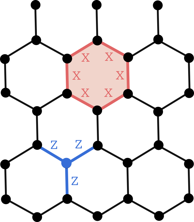
The fact that the stabilizers commute is a direct consequence of the fact that cellulations define valid chain complexes.
We can also consider more exotic cellulations and manifolds. For instance, hyperbolic codes are defined from regular tessellations of hyperbolic manifolds7, such as the following one:
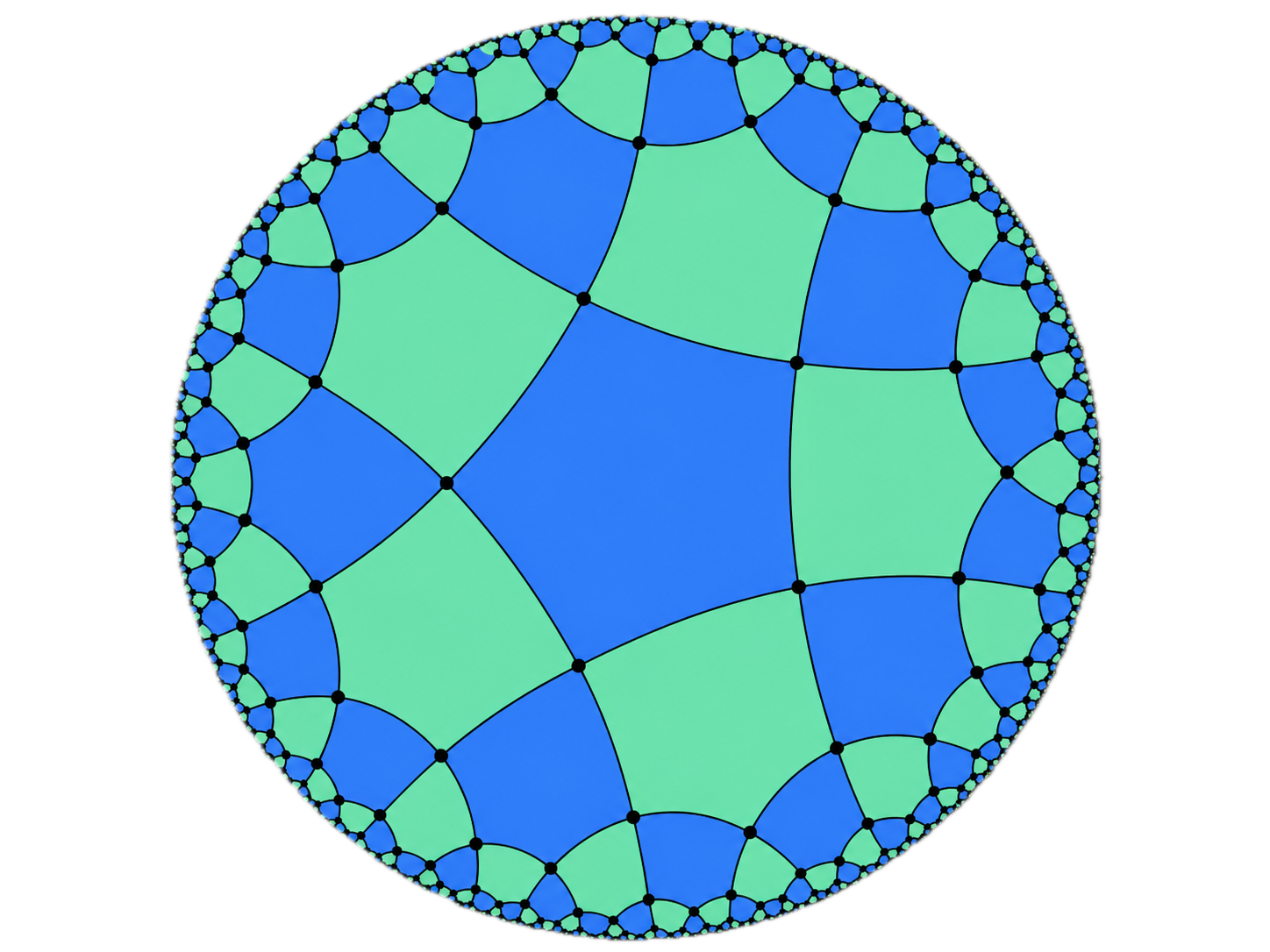
Depending on the chosen boundary conditions, i.e., how different parts of the disk boundary are identified with one another, we can obtain cellulations of different manifolds this way, including high-genus manifolds (obtained by gluing multiple tori together in a suitable way).
What about higher dimensions? Let’s consider a cellulation of a 3D manifold, such as a cubic cellulation of the 3-torus:
represented by a chain complex
\[\begin{aligned} C_3 \xrightarrow{\partial_3} C_2 \xrightarrow{\partial_2} C_1 \xrightarrow{\partial_1} C_0 \end{aligned}\]where \(C_3\) is the space of cubes. We can then extract two possible chain complexes,
\[\begin{aligned} C_3 \xrightarrow{\partial_3} C_2 \xrightarrow{\partial_2} C_1 \end{aligned}\]and
\[\begin{aligned} C_2 \xrightarrow{\partial_2} C_1 \xrightarrow{\partial_1} C_0. \end{aligned}\]These give rise, in principle, to two possible surface codes. In the first case, qubits are placed on faces, with stabilizers on volumes and edges; in the second, qubits are placed on edges, with stabilizers on faces and vertices. However, one can show that \(\partial_3 = \partial_1^T\), meaning that for the cubic lattice these two constructions are in fact equivalent, defining the so-called 3D toric code on a cubic lattice. The 3D toric code is one of my favorite codes, with many cool properties such as the existence of a transversal CCZ gate, and I hope to dedicate a full post to it in the future!
More generally, one can define \(D\)-dimensional toric codes for any \(D\), and depending on the chosen length-2 chain complex, the resulting codes can have different properties. For instance, the 4D toric code can either have a transversal CCCZ gate or serve as a self-correcting quantum memory, depending on this choice.
Conclusion
At the beginning of this post, we asked for a method to construct parity-check matrices satisfying three conditions: orthogonality, sparsity, and non-zero \(k\) with growing \(d\). We found out that algebraic topology provides us with a systematic way to construct orthogonal sparse matrices, by using the boundary operators of manifold cellulations. This works because these boundary operators satisfy the chain complex condition, which is precisely the orthogonality condition required by CSS codes. But we haven’t said anything about the parameters of the codes generated this way: can we guarantee that they have non-zero \(k\) and growing \(d\)? This is what we will explore in the next post, where we will introduce one of the most powerful tools of algebraic topology: the homology group of a chain complex.
Resources
Algebraic topology for quantum error correction:
- PhD Thesis: Quantum error correction in three dimensions and beyond, Chapter 3, by myself.
- PhD Thesis: Homological quantum codes beyond the toric code, Chapter 2, by Nikolas Breuckmann.
- Topological Codes and Computation, by Dan Browne.
General algebraic topology:
- Algebraic Topology, by Allen Hatcher (the bible of the subject).
Solution of the exercise
A natural idea to preserve sparsity, proposed by MacKay et al., 2003, is to consider a random dual-containing LDPC code \(H\) satisfying \(HH^T = 0\), and to set \(H_X = H_Z = H\). However, in this case the rows of \(H\) lie in its own kernel, which contains both stabilizers and logical operators. Due to the randomness of the construction, some stabilizers will almost certainly correspond to low-weight logical operators under the \(X \leftrightarrow Z\) mapping, resulting in a quantum code with constant distance.
-
By topological code, I mean any code family constructed from the cellulation of manifolds of fixed dimension with local stabilizers. In principle, all CSS codes are topological codes, since Freedman and Hastings showed in 2020 that any CSS code can be mapped to a surface code on an 11-dimensional manifold. However, when the most natural way to construct a code is not via the cellulation of a manifold (with local stabilizers), I would not colloquially refer to it as a topological code. ↩︎
-
To be more precise, I should write \((H_X^{(\ell)},H_Z^{(\ell)})\) to emphasize that we are dealing with a family of codes indexed by an integer \(\ell\), rather than a single code (e.g. \(\ell\) would correspond to the lattice size for the surface code). The parameters of the code family could then be written \([[n_\ell,k_\ell,d_\ell]]\). I omit this index here and throughout the post to avoid overloading the notation, as it should be clear from context when there is an implicit dependence on \(\ell\). ↩︎
-
To see the difficulty, suppose we take \(H_X\) to be a random sparse parity-check matrix, defining a good classical LDPC code. Then, to satisfy the orthogonality condition \(H_X H_Z^T = 0\), the rows of \(H_Z\) must lie in the kernel of \(H_X\). But for a good LDPC code, all non-zero codewords (i.e., elements of the kernel) typically have weight scaling as \(O(n)\), which prevents \(H_Z\) from being sparse. ↩︎
-
A more common way to define cellulations in modern algebraic topology is via CW-complexes. This is what you will find for instance in Hatcher, the bible of algebraic topology. This method often provides much smaller cellulations of a given manifold, by allowing objects such as monogons (a point with a self-loop and a face inside) and bigons (two points connected by two edges and a face instead) to serve as cells, even though these are not strictly-speaking polytopes. With CW-complexes, a torus can for instance be cellulated using only one vertex, two edges and one face (you can see it as a 1x1 lattice with periodic boundary conditions), while the simplest polytope-based cellulation requires four faces, eight edges, and four vertices (a 2x2 lattice with periodic boundary conditions), due to the requirements for our maps to be homeomorphisms. However, CW-complexes are also more complicated to define rigorously, and in practice, polytope cellulations are sufficient for most applications in QEC. ↩︎
-
This can be made rigorous, by defining the manifold as the square \(S=[0,1]^2\) quotiented by an equivalence relation \(\sim\) such that top-bottom boundaries are equivalent, i.e., \((x,0) \sim (x,1)\) for all \(x \in [0,1]\), and left-right boundaries are equivalent, i.e., \((0,y) \sim (1,y)\) for all \(y \in [0,1]\). We previously encountered the notion of quotient, defining the quotient of a group (the logicals) by a subgroup (the stabilizers). The idea is similar for topological spaces: the quotient \(\mathcal{M}=S/\sim\) of the topological space \(S\) (our square) by the equivalence relation \(\sim\) is formally defined as a space of sets (called cosets) such that each coset contains equivalent points. In our case, cosets corresponding to points in the bulk of our square are singleton, e.g. \(\{ (0.5, 0.2) \}\), while cosets corresponding to points at the boundaries contain either two elements, e.g. \(\{ (0,0.5), (1,0.5) \}\) or four for the corners, e.g. \(\{(0,0),(0,1),(1,0),(1,1)\}\). We can make this quotient a topological space by defining the neighborhood of points at the boundary to correspond to the union of neighborhoods on both sides, and one can then verify that the resulting space is indeed a manifold, fulfilling all the properties discussed above. ↩︎
-
For a rigorous proof of this fact, see Lemma 2.9 of Niko Breuckmann’s PhD thesis. ↩︎
-
A tessellation is a cellulation in which each map from a polytope to the manifold is an isometry, i.e., it preserves angles and distances. A regular tessellation is a tessellation that uses a single type of polytope, and has the same number of edges meeting at each vertex. For instance, regular tessellations of the plane \(\mathbb{R}^2\) are made from polygons of the same type and size, and one can prove that only three types of regular tessellations of the plane exist: those made from equilateral triangles, squares, or hexagons. In the hyperbolic plane, such as the Poincaré disk model shown in the figure, we choose a metric such that the distance of edges close to the boundary have a much higher length than it seems visually (i.e., when measured with a Euclidean metric on the disk). The depicted cellulation is therefore a regular cellulation with pentagons and degree-4 vertices, where all the 2-cells actually have the same area with respect to the hyperbolic metric. ↩︎