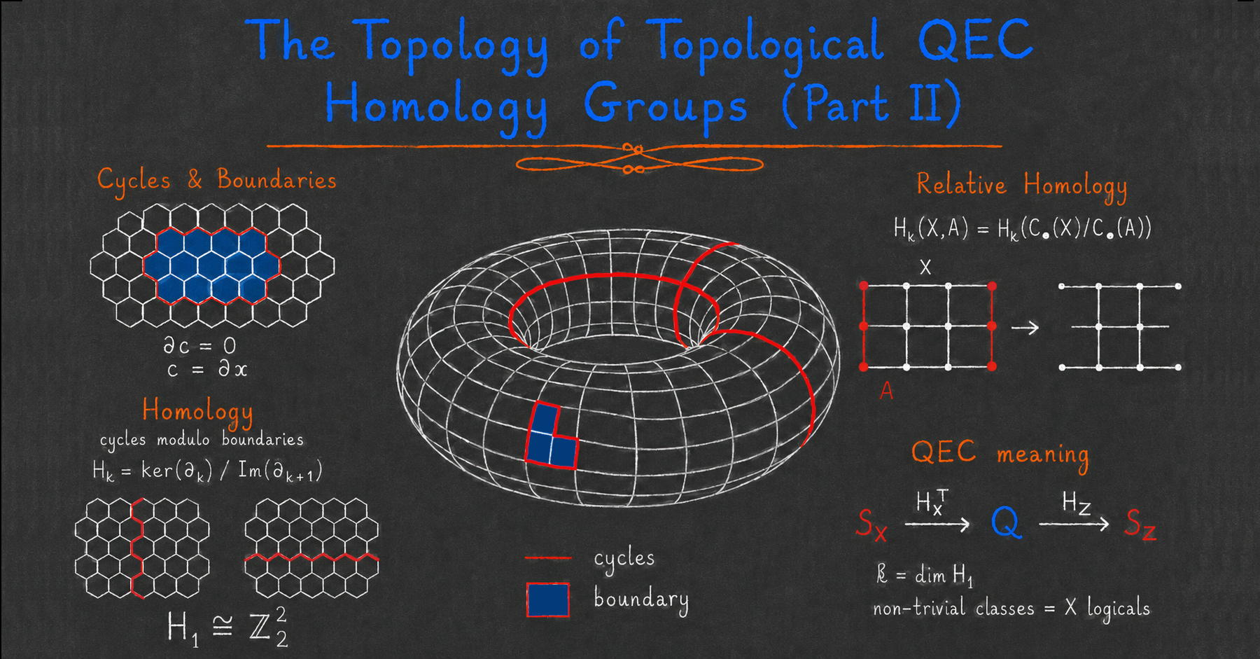
The topology of topological QEC II — Homology groups
In the previous post, we introduced algebraic topology through one of its most important objects: chain complexes. We saw how chain complexes can be constructed from cellulations of manifolds and how they give rise to CSS codes. But the main reason both mathematicians and quantum error correctors like chain complexes is that they allow us to define homology groups!
From a mathematical point of view, homology groups provide topological invariants of manifolds: quantities that do not depend on the particular cellulation we choose and do not change when the manifold is continuously deformed. From a quantum error correction point of view, they give us the number of logical qubits of a code and help us understand the structure of logical operators.
In Part II of our series on topological quantum error correction, we will introduce homology groups and explain their interpretation in the context of quantum error correction. This post is filled with examples and exercises, which should hopefully give you a good intuition for what these objects are and how to use them to calculate useful quantities.
The next and final post in this series will focus on cohomology groups. These are closely related to homology groups, and they will allow us to develop a fuller understanding of the structure of logical operators in CSS codes. They will also give us many useful theorems and tools for calculating the homology of manifolds and constructing logical gates in quantum codes.
But let’s not get ahead of ourselves. Let’s start with homology groups!
Cycles and boundaries
Let’s start by introducing some important terminology. Given a length-\(D\) chain complex
\[\begin{aligned} C_D &\xrightarrow{\partial_D} C_{D-1} \xrightarrow{\partial_{D-1}} \cdots \xrightarrow{\partial_2} C_1 \xrightarrow{\partial_1} C_0 , \end{aligned}\]and \(k \in \{0,\ldots,D\}\), a \(\bm{k}\)-chain is an element of \(C_k\). For instance, if the chain complex comes from a cellulation of a manifold, a \(0\)-chain is a set of vertices, represented as a binary vector whose support is that set. Similarly, a \(1\)-chain is a set of edges, a \(2\)-chain is a set of faces, and so on.
For any \(k \in \{0,\ldots,D-1\}\), a \(\bm{k}\)-boundary is an element of \(\Im(\partial_{k+1})\). In other words, a \(k\)-boundary is a \(k\)-chain that can be written as the boundary of a \((k+1)\)-chain. For instance, in a cell complex, a \(1\)-boundary is a set of edges that forms the boundary of some faces, and a \(0\)-boundary is a set of vertices that forms the boundary of some edges.
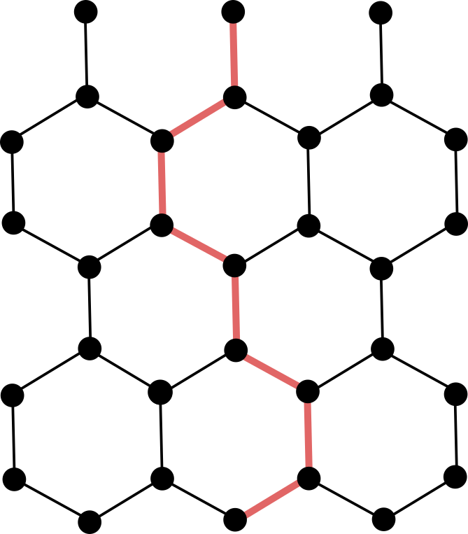
Here is an example of a \(1\)-boundary in a hexagonal cellulation of a torus, where the left-right and top-bottom boundaries are identified:
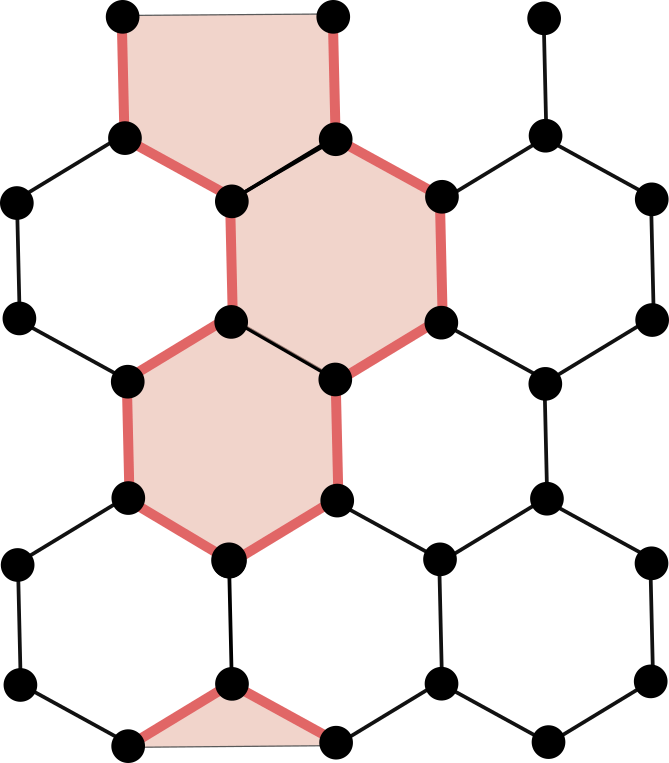
This is a set of \(14\) edges, or rather a vector with \(14\) ones, equal to the boundary of a chain made of three faces. In other words, it is the image of these three faces under the boundary map \(\partial_2\). Similarly, the following set of two vertices is a \(0\)-boundary: it is the boundary of a path made of three edges, or equivalently the image of those edges under \(\partial_1\).
We now define a \(\bm{k}\)-cycle as an element of \(\ker(\partial_k)\), for any \(k \in \{1,\ldots,D\}\). In other words, a \(k\)-cycle is a \(k\)-chain with no boundary. For instance, in a 2D cell complex, a \(1\)-cycle is a set of edges forming closed loops, and a \(2\)-cycle is a set of faces whose total boundary cancels.
Returning to our hexagonal cellulation example, what would be a \(2\)-cycle? There is exactly one non-zero \(2\)-cycle, formed by all the faces, i.e. the all-one vector:
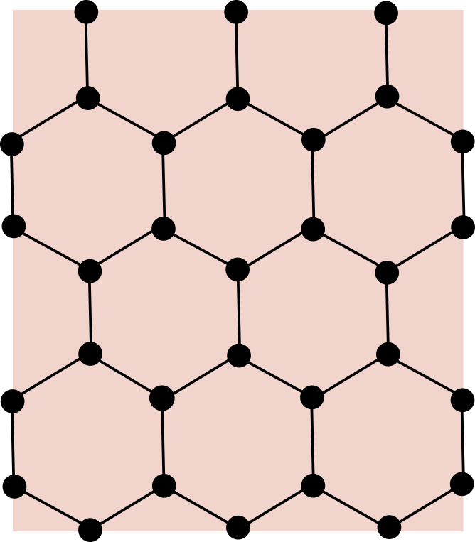
If we had instead chosen a cellulation of a disconnected manifold, such as two disconnected tori, we would have one independent \(2\)-cycle per connected component, formed by taking all the faces of that component. Equivalently, for a closed 2D manifold, the dimension of \(\ker(\partial_2)\) is equal to the number of connected components of the manifold.
What about \(1\)-cycles? The first thing to notice is that the \(1\)-boundaries of our cellulation are also \(1\)-cycles: since they form closed loops, they have no boundary.
Is it always the case that \(k\)-boundaries are \(k\)-cycles for any \(k \geq 1\), even for a generic chain complex? Yes, and this is exactly the defining condition of a chain complex. Recall the chain complex condition:
\[\begin{aligned} \partial_{k} \circ \partial_{k+1} = 0 . \end{aligned}\]This can also be written as
\[\begin{aligned} \Im(\partial_{k+1}) \subseteq \ker(\partial_k), \end{aligned}\]which means precisely that all \(k\)-boundaries are also \(k\)-cycles for \(k \geq 1\). This should make intuitive sense: the chain complex condition says that the boundary of a boundary is always empty. Therefore, if a chain is itself a boundary, then it has no boundary, and hence it is a cycle.
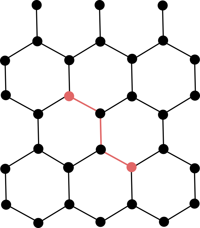
However, not all \(1\)-cycles are \(1\)-boundaries. For instance, the following set of edges is a \(1\)-cycle but not a \(1\)-boundary:
This observation is the starting point of homology theory: homology measures cycles that are not boundaries.
Homology groups
The \(\bm{k}\)-th homology group of a chain complex \(C_\bullet\) is defined as the quotient vector space
\[H_k(C_\bullet) = \ker(\partial_k) / \Im(\partial_{k+1})\]for all \(k \in \{0,\ldots,D\}\). The quotient is well-defined because, as we saw, \(\Im(\partial_{k+1}) \subseteq \ker(\partial_k)\).
To make the definition work for \(k=0\) and \(k=D\) as well, we extend the chain complex by adding zero vector spaces at both ends:
\[\begin{aligned} C_{D+1}=0 &\xrightarrow{\partial_{D+1}=0} C_D \xrightarrow{\partial_D} C_{D-1} \xrightarrow{\partial_{D-1}} \cdots \xrightarrow{\partial_2} C_1 \xrightarrow{\partial_1} C_0 \xrightarrow{\partial_{0}=0} C_{-1}=0 . \end{aligned}\]Here, \(\partial_{D+1}\) is the unique map from \(C_{D+1}=0\) to \(C_D\), sending the zero vector of \(C_{D+1}\) to the zero vector of \(C_D\). Similarly, \(\partial_0\) is the unique map from \(C_0\) to \(C_{-1}=0\), sending every vector of \(C_0\) to the zero vector of \(C_{-1}\).
The \(k\)-th homology group can be thought of as the space of \(k\)-cycles up to \(k\)-boundaries. Since it is a quotient of vector spaces, it also has the structure of a vector space. The name “group” is still correct, since vector spaces are in particular abelian groups, but it is mainly a historical convention. Nowadays, in our setting, it is often more useful to think of homology groups as vector spaces, or more generally as \(R\)-modules over some ring \(R\) 1.
Two \(k\)-cycles are said to be homologically equivalent if they belong to the same coset, i.e. if they differ by a \(k\)-boundary. In other words, two \(k\)-cycles are homologically equivalent if one can be transformed into the other by adding a \(k\)-boundary. Nonzero elements of the homology group are homology classes that cannot be reduced to zero by adding boundary elements.
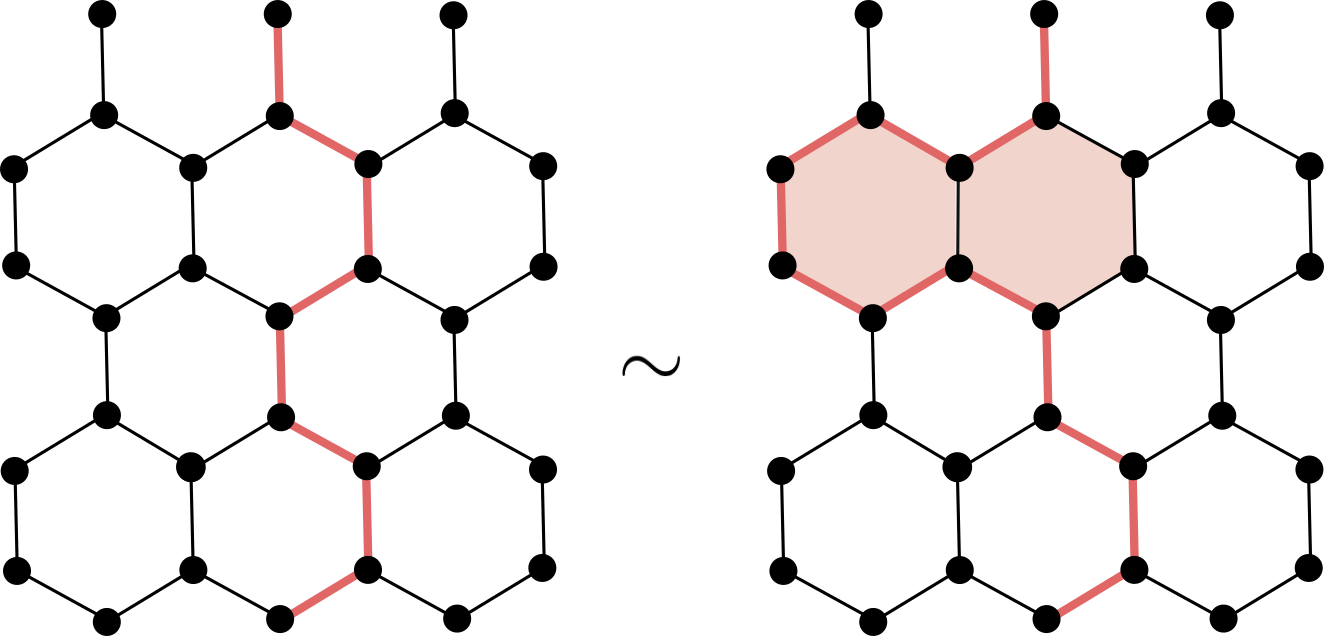
For instance, in our hexagonal cellulation example, these two \(1\)-cycles, shown in red, are homologically equivalent, since one can be obtained from the other by adding the boundary of the two red plaquettes:
They are also non-trivial: you cannot reduce them to zero by adding any \(1\)-boundary. A homologically distinct non-trivial coset is represented by the following \(1\)-cycle:
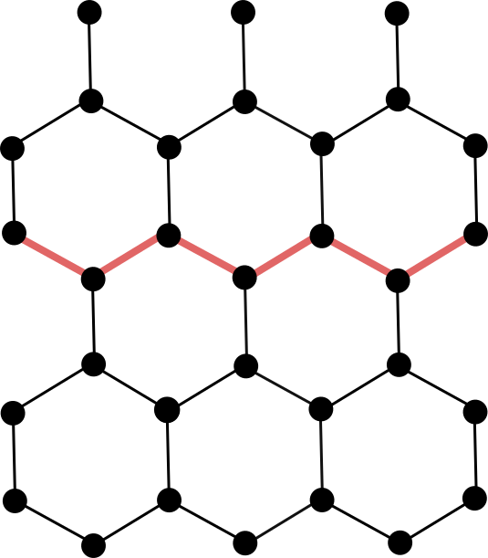
What is the dimension of the first homology group \(H_1(C_\bullet)\) in our example? Since there are two independent non-trivial homology classes, corresponding to loops going around the torus horizontally and vertically, the homology group has dimension \(2\). We could prove this by computing the kernel and image of the boundary maps explicitly, since they are just matrices, and using the formula for the dimension of a quotient space:
\[\begin{aligned} \dim(H_k(C_\bullet)) = \dim(\ker(\partial_k)) - \dim(\Im(\partial_{k+1})) . \end{aligned}\]As we will see later, we can also deduce this directly from the fact that our chain complex corresponds to a cellulation of the \(2\)-torus.
Since any \(\mathbb{Z}_2\)-vector space of dimension \(n\) is isomorphic to \(\mathbb{Z}_2^n\), we can write
\[\begin{aligned} H_1(C_\bullet) \cong \mathbb{Z}_2^2 . \end{aligned}\]After choosing the horizontal and vertical homology classes as generators, we can identify \(H_1(C_\bullet)\) with \(\mathbb{Z}_2^2\). Under this identification, the homology class \((1,0)\) is represented by a horizontal loop around the torus, the class \((0,1)\) is represented by a vertical loop, and the class \((1,1)\) is represented by the sum of these two loops.
Let’s now discuss the \(0\)-th and \(D\)-th homology groups. By definition, we have
\[\begin{aligned} H_0(C_\bullet) &= \ker(\partial_0) / \Im(\partial_1) = C_0 / \Im(\partial_1), \\ H_D(C_\bullet) &= \ker(\partial_D) / \Im(\partial_{D+1}) = \ker(\partial_D) / \{0\} = \ker(\partial_D), \end{aligned}\]since \(\ker(\partial_0) = C_0\) and \(\Im(\partial_{D+1}) = \{0\}\).
These homology groups have a simple interpretation in the cell complex case. The \(0\)-th homology group consists of \(0\)-chains, i.e. sets of vertices, up to the equivalence relation that identifies two vertices if they are connected by a path. Indeed, \(0\)-boundaries are boundaries of \(1\)-chains, i.e. sets of edges, so adding a \(0\)-boundary allows us to move vertices along paths in the cellulation. The dimension of \(H_0(C_\bullet)\) is therefore exactly the number of connected components of the manifold: vertices in the same connected component are homologically equivalent, while vertices in different connected components are not.
What about the \(D\)-th homology group? It consists of all \(D\)-chains with no boundary. In the case of a closed \(D\)-dimensional manifold, these are generated by taking the sum of all \(D\)-cells in each connected component. Thus, \(H_D(C_\bullet)\) also has one generator per connected component.
The fact that \(H_D(C_\bullet)\) and \(H_0(C_\bullet)\) have the same dimension, for closed manifolds, is a special case of a more general result called Poincaré duality, which we will see in the post on cohomology.
QEC interpretation
Let’s now return to quantum error correction and interpret the objects we have just introduced. Consider the chain complex
\[\begin{aligned} \mathcal{S}_X &\xrightarrow{H_X^T} \mathcal{Q} \xrightarrow{H_Z} \mathcal{S}_Z . \end{aligned}\]The space of \(1\)-cycles is given by \(\ker(H_Z)\), and can be interpreted as the space of \(X\) operators that commute with all \(Z\) stabilizers. The space of \(1\)-boundaries is given by \(\Im(H_X^T)\), and can be interpreted as the space of \(X\) stabilizers. The first homology group is therefore
\[\begin{aligned} H_1(C_\bullet) = \ker(H_Z) / \Im(H_X^T), \end{aligned}\]and can be interpreted as the space of \(X\) logical cosets: \(X\) operators that commute with all \(Z\) stabilizers, up to equivalence by \(X\) stabilizers. As we saw in the previous post, the dimension of this space is exactly the number \(k\) of logical qubits of the code.
What about \(Z\) logical cosets? Do they have a homological interpretation as well? Yes: they correspond to the homology group of a different complex, where the roles of \(H_X\) and \(H_Z\) are swapped:
\[\begin{aligned} \mathcal{S}_Z &\xrightarrow{H_Z^T} \mathcal{Q} \xrightarrow{H_X} \mathcal{S}_X . \end{aligned}\]This new complex is called the cochain complex, and it will be the main protagonist of the next post in this series.
Finally, can the distance be given a homological interpretation as well? If we assign a weight to elements of \(C_1\), for instance their Hamming weight, then the \(X\) distance of the code is the weight of the smallest non-trivial representative of \(H_1(C_\bullet)\). Similarly, the \(Z\) distance is obtained from the cochain complex.
However, while homology groups are topological invariants of manifolds, as we will see in the next section, the distance is not. It can vary significantly between different cellulations of the same manifold. Moreover, homological algebra does not provide an obvious general tool for computing the distance.
When dealing with cellulations of manifolds, the main area of mathematics that says something about distance is systolic geometry, which studies the length of the shortest non-contractible loop in a manifold. However, systolic geometry mainly gives general laws for how the distance can grow with the size of the code, sometimes leading to no-go theorems. It does not usually provide a practical tool for computing the distance of a specific cellulation, and it does not generalize easily beyond manifolds.
In most cases, distance calculations need to be carried out explicitly for the specific code at hand.
Homology of a manifold
A landmark result of algebraic topology is that the homology groups of a manifold cellulation are independent of the particular cellulation. They only depend on the underlying manifold, and will also stay the same when transforming the manifold via a homeomorphism (continuous bijection with continuous inverse) or homotopy equivalence (progressive continuous deformation of the manifold). For instance, any cellulation of the 2-torus will have \(H_1(C_\bullet)=\mathbb{Z}_2^2\) as its first homology group. This was not a property of the specific hexagonal cellulation we chose, but a consequence of the fact that we had a 2D lattice with periodic boundary conditions, i.e. a cellulation of a 2-torus.
One way to formalize this theorem is by defining a different notion of homology, called singular homology. Intuitively, singular homology is the homology of an infinitely fine-grained cellulation of the manifold, where we allow \(0\)-chains to be any point of the manifold, \(1\)-chains to be any curve, \(2\)-chains to be any surface, and so on. Here are examples of singular chains (in red) on a torus:
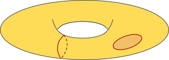
where we have one non-trivial singular \(1\)-cycle (going around the torus) and one trivial one, whose boundary (a \(2\)-chain) is represented in light red.
The way singular homology works is by defining a chain complex whose space \(C_k\) is the infinite-dimensional vector space of all continuous maps from the \(k\)-simplex to the manifold. For instance, a singular \(1\)-chain of the torus would be a map from a segment (1-simplex) to a line on the torus. A \(1\)-cycle would be a map from the segment to a loop on the torus. The details of this construction are not too important for us. The key point is that the homology groups of a manifold cellulation are isomorphic to the singular homology groups of the underlying manifold, and therefore to the homology groups obtained from any other cellulation of the same manifold. In other words, the homology groups of a cell complex only depend on the underlying manifold. For a formal version of this result, see for instance Hatcher’s book, Theorem 2.35. We will denote the homology groups of a manifold \(\mathcal{M}\) by \(H_i(\mathcal{M})\).
The nice thing about this result is that algebraic topology has plenty of methods to calculate the homology of a manifold. The most direct way is to take the smallest cellulation you can find of your manifold, write down boundary matrices, kernels, images, and homology groups for this cellulation, and it will tell you the homology of the manifold. This is pure linear algebra on small matrices.
Another way is to use homotopy equivalences to map the manifold to a simpler one whose homology is easy to compute. For instance, if the manifold can be continuously deformed to a point (we say that the manifold is contractible), then all its \(k\)-homology groups vanish for \(k \geq 1\). You can use this to prove that any \(n\)-dimensional hypercube (or equivalently, the disk \(D^n\)) has trivial homology beyond the zeroth homology (we will use this fact later in the post, when discussing open boundaries).
Another convenient calculation method is to write your manifold as a product of simpler manifolds, and use a formula (called the Künneth formula) to compute the homology of the product from the homology of the factors. See Exercise 3 below for an example of this.
And this is only the tip of the iceberg! There are many more tools to compute homology groups: the Mayer-Vietoris sequence (if you can decompose your manifold as a union of simpler manifolds), the long exact sequence in relative homology (see Exercise 6), spectral sequences (recently used to prove the existence of self-correction quantum memory in 3D), and so on.
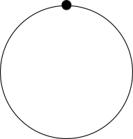
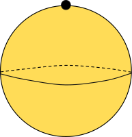
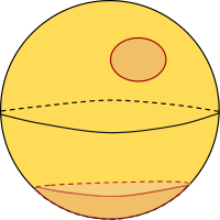
Two important examples of homology calculation include the \(D\)-sphere and \(D\)-torus. We derive their homology groups in the following two exercises.
Another cool result of homology theory applied to manifolds is the existence of combinatorial invariants of cellulations, such as the Euler characteristic. Given a cell complex \(C_\bullet\), it is defined as
\[\begin{aligned} \chi = \sum_{k=0}^D (-1)^k \dim(C_k) \end{aligned}\]It turns out that \(\chi\) only depends on the manifold, and can be computed from the dimensions of the different homology groups. Let \(b_k = \dim(H_k(C_\bullet))\) be the dimension of the \(k\)-th homology group, also called the \(\bm{k}\)-th Betti number. Then, we have
\[\begin{aligned} \chi = \sum_{k=0}^D (-1)^k b_k \end{aligned}\]The proof is actually not too difficult, it is a direct consequence of our definitions, plus a tiny bit of linear algebra (this is the cool thing about reducing topology to linear algebra!). It is a good exercise to check that you have integrated all the concepts so far!
As an example, for a connected 2D manifold, we know that \(b_0 = b_2=1\). Moreover, by construction of the cell complex, \(V=\dim(C_0)\) is the number of vertices of the cellulation, \(E=\dim(C_1)\) is the number of edges, and \(F=\dim(C_2)\) is the number of faces. We therefore have:
\[\begin{aligned} V - E + F = 2 - b_1 \end{aligned}\]For instance, the 2-sphere has \(b_1=0\) (see Exercise 2 above), and so \(V - E + F = 2\). The formula was originally found in this form by Euler, when studying combinatorial invariants of polyhedra (a polyhedron can be seen as a cellulation of the sphere). For instance, a cube has \(V=8\) vertices, \(E=12\) edges, and \(F=6\) faces, and indeed we have \(8 - 12 + 6 = 2\).
The Euler characteristic formula is frequently used in topological quantum error correction. The following exercise gives an example in the context of the 2D color code.
Where does this leave us in our quest to find useful quantum error-correcting codes? Our goal was to find families of LDPC codes with parameters \([[n,k,d]]\) such that \(k\) is non-zero and \(d\) grows with \(n\). We described in the previous post a potential recipe to construct such a code: take a family of manifold cellulations and an integer \(\ell\), and extract from it the length-2 chain complex with \(\ell\)-cells as qubits. We now have a new guarantee on such a code: if the manifold has \(b_\ell > 0\), then the code has \(k=b_\ell > 0\). If the cellulation family is constructed from a fixed manifold by progressively refining a small cellulation, then the distance will also usually grow, with the precise distance formula depending on the specific cellulation chosen.
Manifolds with boundary and relative homology
There is still one big element missing from our discussion so far: how can we understand surface codes with open boundaries in the language of homology? We saw in the surface code post that by replacing the periodic boundaries by opposite smooth and rough boundaries, we can get a planar code with \(k=1\). Could we have constructed this code from purely algebraic-topological considerations, and calculated \(k\) as the homology of a certain manifold?
It turns out that algebraic topology does provide us with exactly the right notion to describe surface codes with boundaries: relative homology. Consider a manifold \(\mathcal{M}\) (possibly with boundary) and a cellulation \(X\) of \(\mathcal{M}\) described by the chain complex
\[\begin{aligned} C_D(X) &\xrightarrow{\partial^X_D} C_{D-1}(X) \xrightarrow{\partial^X_{D-1}} \cdots \xrightarrow{\partial^X_2} C_1(X) \xrightarrow{\partial^X_1} C_0(X) \end{aligned}\]Now, consider a submanifold \(\mathcal{N} \subseteq \mathcal{M}\) (usually, with \(\mathcal{N} \subset \partial \mathcal{M}\), but not necessarily) with the induced cellulation \(A\) obtained by taking all cells of \(X\) that are contained in \(\mathcal{N}\). It is described by the chain complex
\[\begin{aligned} C_D(A) &\xrightarrow{\partial^A_D} C_{D-1}(A) \xrightarrow{\partial^A_{D-1}} \cdots \xrightarrow{\partial^A_2} C_1(A) \xrightarrow{\partial^A_1} C_0(A) \end{aligned}\]We can then define the relative chain complex as
\[\begin{aligned} C_D(X,A) &\xrightarrow{\partial_D} C_{D-1}(X,A) \xrightarrow{\partial_{D-1}} \cdots \xrightarrow{\partial_2} C_1(X,A) \xrightarrow{\partial_1} C_0(X,A) \end{aligned}\]where \(C_k(X,A) = C_k(X) / C_k(A)\) is the quotient of the vector space of \(k\)-chains of \(X\) by the subspace of \(k\)-chains of \(A\). Intuitively, the relative chain complex is obtained by setting the submanifold \(\mathcal{N}\) to zero. Elements of \(\ker(\partial_k)\) are then called relative \(k\)-cycles, and elements of \(\Im(\partial_{k+1})\) are called relative \(k\)-boundaries. The relative homology groups are defined as the quotient of relative cycles by relative boundaries:
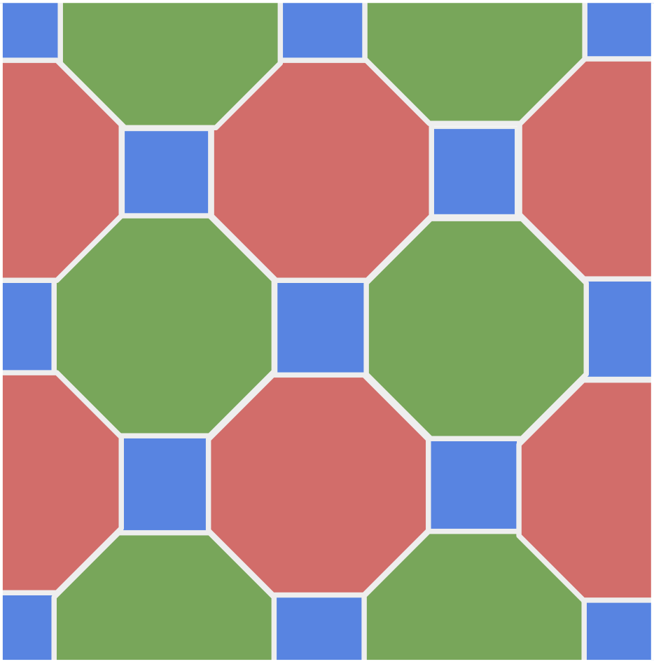
\[\begin{aligned} H_k(X,A) = \ker(\partial_k) / \Im(\partial_{k+1}). \end{aligned}\]Let’s see if we can obtain the open surface code from this construction. Let’s start with the following cellulation \(X\) of the disk \(D^2\) (which is topologically equivalent to a square or rectangle):
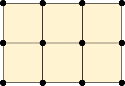
Note that the first homology of that cellulation is zero: as discussed before, any disk is contractible and therefore has trivial homology beyond the zeroth homology. It should also be clear from the picture that any \(1\)-cycle in such a cellulation is the boundary of a collection of faces, so there are no non-trivial homology classes. Now, let’s consider the submanifold consisting of the left and right boundaries of the rectangle, highlighted in red in the figure below:
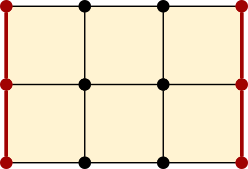
Setting those boundaries to zero, which is equivalent to removing the corresponding vertices and edges from the cell complex, then gives us the following relative complex:
It’s exactly our surface code with rough and smooth boundaries! So, how can we show that the first homology group of this relative complex has dimension one? As before, it is possible to show that the relative homology group is also cellulation-independent, meaning that we can simply take the smallest cellulation of the square and compute its relative homology using linear algebra.
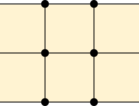
Let’s pick the following cellulation, and remove the left and right boundaries:
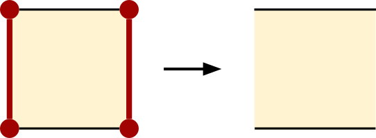
The resulting relative complex has zero vertices, two edges, and one face, giving the complex
\[\begin{aligned} \mathbb{Z}_2 &\xrightarrow{\partial_2} \mathbb{Z}_2^2 \xrightarrow{\partial_1} 0 \end{aligned}\]with \(\partial_2 = \begin{pmatrix} 1 \\ 1 \end{pmatrix}\) and \(\partial_1 = 0\). The space of relative \(1\)-cycles is then given by \(\ker(\partial_1) = \mathbb{Z}_2^2\), and the space of relative \(1\)-boundaries is given by \(\Im(\partial_2) = \mathbb{Z}_2\), so the first relative homology group has dimension one, as expected.
The following exercise shows that this idea generalizes very well to any \(D\)-dimensional hypercube, by setting two opposite sides to zero. This builds the open boundary version of the \(D\)-dimensional toric code, which has \(k=1\) for any dimension \(D\) (the 3D surface code is an example of this).
Conclusion
Well done for surviving this long post! You’re now familiar with one of the most profound notions of modern mathematics, and how to use it to concretely calculate the number of logical qubits of a topological quantum code! This should already give you a good understanding of why the 2D surface code magically worked so well, and how to generalize it to other manifolds and dimensions.
However, we’re still missing a few things. We saw that the homology of our CSS chain complex really tells us about the \(X\) logicals of the code. This is enough to tell us how many logical qubits we have, but to characterize \(Z\) logicals as well, we need to introduce a new notion, called cohomology. We can then show for instance that for a manifold cellulation, \(Z\) logicals are given by the homology of the dual lattice (remember the dual lattice from the surface code post?). We can also show that there exists a basis of logical operators such that each logical \(X\) operator anticommutes with exactly one logical \(Z\) operator, and commutes with all the others. Cohomology has also become trendy in QEC recently due to the construction of certain types of logical gates using cup products, a concept that belongs to cohomology theory. There are therefore many reasons to learn cohomology, and I am looking forward to telling you all about it in the next post!
Resources
Algebraic topology for quantum error correction:
- PhD Thesis: Quantum error correction in three dimensions and beyond, Chapter 3, by myself.
- PhD Thesis: Homological quantum codes beyond the toric code, Chapter 2, by Nikolas Breuckmann.
- Topological Codes and Computation, by Dan Browne.
General algebraic topology:
- Algebraic Topology, by Allen Hatcher (the bible of the subject).
Solution of the exercise
-
An \(R\)-module is a generalization of a vector space in which the coefficients form a ring \(R\) rather than a field. The key difference is that, in a general ring, nonzero elements need not be invertible. An archetypal example is the \(\mathbb{Z}\)-module \(\mathbb{Z}^n\), the set of \(n\)-dimensional vectors with integer coefficients. This is a module but not a vector space, since most elements of \(\mathbb{Z}\), apart from \(1\) and \(-1\), do not have an inverse in \(\mathbb{Z}\). Many familiar tools from linear algebra, such as Gaussian elimination or dimension-counting arguments, do not carry over directly to general \(R\)-modules. However, algebraic topology is often developed using \(\mathbb{Z}\)-modules, because integer coefficients keep track of cycles with integer multiplicities (think of loops going around multiple times around a hole) and can capture phenomena, such as torsion, that disappear over fields. In contrast, when restricting to field coefficients such as \(\mathbb{Z}_2\), many results from algebraic topology and homological algebra become much simpler. ↩︎