The topology of topological QEC III — Cohomology groups
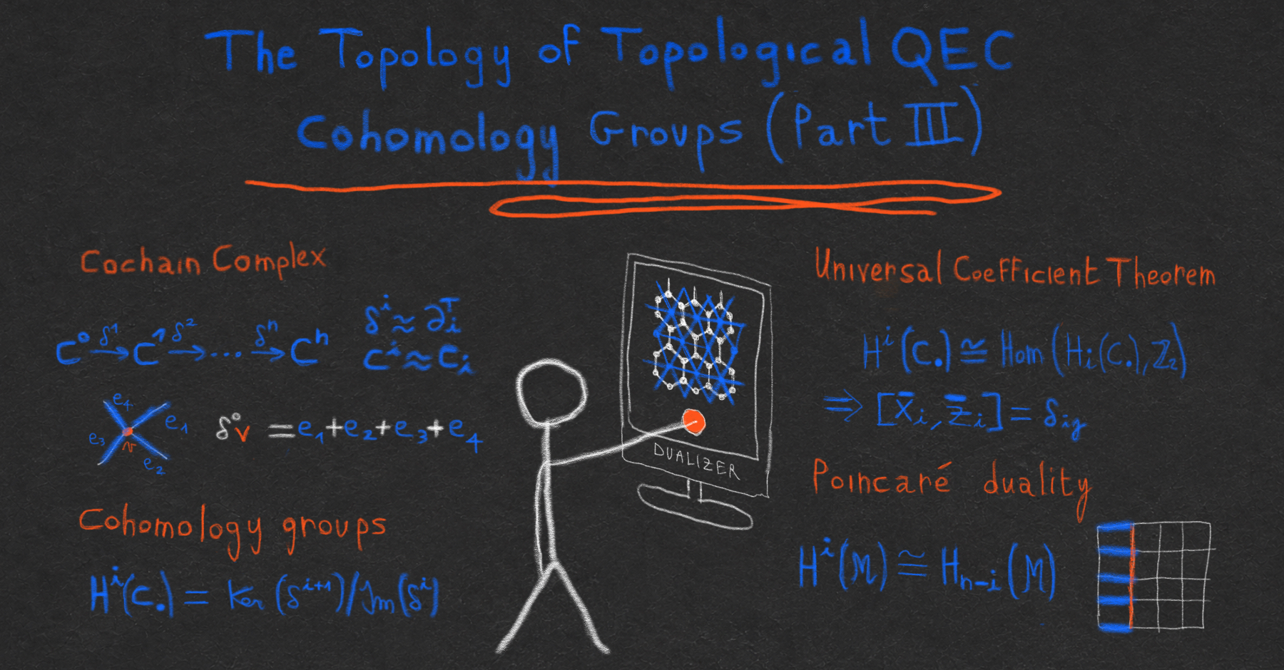
In the two previous posts, we learned about chain complexes and their homology groups. We are now ready for another foundational concept needed to understand QEC from a topological perspective: in this copost, we will dive into cohomology!
When learning about the surface code, we saw that \(Z\) logical operators can be seen as loops in a dual lattice, constructed by replacing faces of the original lattice by vertices, vertices by faces, and edges by orthogonal ones. What is the interpretation of this construction from an algebraic topology perspective? It turns out that this dual lattice construction is an instance of a more general construction called the cochain complex, which leads to the definition of cohomology groups. Cohomology groups are closely related to homology groups, and as we will see, can be interpreted as \(Z\) logical cosets if the homology groups correspond to \(X\) logical cosets.
We will first introduce the cochain complex and cohomology groups, and then see two important theorems that relate homology and cohomology groups: the universal coefficient theorem and Poincaré duality. These tools will help us characterize the space of logical operators, and provide a helpful way to compute the number of logical qubits of some topological codes. Let’s get going!
Cochain complex and cohomology groups
Given a length-\(D\) chain complex \(C_\bullet\)
\[\begin{aligned} C_D &\xrightarrow{\partial_D} C_{D-1} \xrightarrow{\partial_{D-1}} \cdots \xrightarrow{\partial_2} C_1 \xrightarrow{\partial_1} C_0 \end{aligned}\]we can construct a new length-\(D\) complex, called the cochain complex \(C^\bullet\), as
\[\begin{aligned} C^0 &\xrightarrow{\delta^1} C^1 \xrightarrow{\delta^2} \cdots \xrightarrow{\delta^{D-1}} C^{D-1} \xrightarrow{\delta^{D}} C^D \end{aligned}\]where \(C^i\) is the dual of \(C_i\), that is, the set of linear maps from \(C_i\) to \(\mathbb{Z}_2\):
\[\begin{aligned} C^i = \text{Hom}(C_i, \mathbb{Z}_2) \end{aligned}\]and the coboundary operators \(\delta^i: C^{i-1} \to C^i\) are defined as
\[\begin{aligned} \delta^i(f) = f \circ \partial_i. \end{aligned}\]Let’s interpret these new objects. An element \(f \in C^i\), that we call an \(\bm{i}\)-cochain, is a map that outputs a bit for every \(i\)-chain. Given a basis of \(i\)-chains \(c_1,\ldots,c_m \in C_i\), we can interpret the function \(f\) as a selection of basis elements: \(f(c_k)=1\) if \(c_k\) is selected, and \(f(c_k)=0\) otherwise. As a linear map from an \(m\)-dimensional space to a \(1\)-dimensional space, we can also write \(f\) as an \(1 \times m\) matrix
\[\begin{aligned} f = \begin{pmatrix} f_1 & f_2 & \cdots & f_m \end{pmatrix} \end{aligned}\]where \(f_k=f(c_k)\). Cochains can therefore be interpreted simply as row vectors with a \(1\) in column \(k\) if the basis chain \(c_k\) is selected by \(f\). Contrast this with the interpretation of chains as column vectors, with a \(1\) in row \(k\) if \(c_k\) is in the basis decomposition of the chain. We can make the correspondence between chains and cochains concrete by constructing an isomorphism \(\psi\) from \(C^i\) to \(C_i\), which maps row vectors to column vectors:
\[\begin{aligned} \psi:\: \begin{pmatrix} f_1 & f_2 & \cdots & f_m \end{pmatrix} \mapsto \begin{pmatrix} f_1 \\ f_2 \\ \vdots \\ f_m \end{pmatrix} \end{aligned}\]In the finite-dimensional setting we care about here, one can therefore identify the space \(C^i\) with \(C_i\), and every cochain \(f \in C^i\) with a corresponding chain \(\tilde{f} \in C_i\).
Let’s now move on to the coboundary operators. These send row vectors of \(C^{i-1}\) to row vectors of \(C^i\) by composing them with the boundary operator \(\partial_i\):
\[\begin{aligned} \delta^i:\: \begin{pmatrix} f_1 & f_2 & \cdots & f_m \end{pmatrix} \mapsto \begin{pmatrix} f_1 & f_2 & \cdots & f_m \end{pmatrix} \begin{pmatrix} & & \\ & \partial_i & \\ & & \end{pmatrix} \end{aligned}\]It’s easy to check that these indeed obey the chain complex condition:
\[\begin{aligned} \delta^{i+1} \delta^i f = \begin{pmatrix} f_1 & f_2 & \cdots & f_m \end{pmatrix} \begin{pmatrix} & & \\ & \partial_i & \\ & & \end{pmatrix} \begin{pmatrix} & & \\ & \partial_{i+1} & \\ & & \end{pmatrix} = 0 \end{aligned}\]since \(\partial_{i} \partial_{i+1} = 0\).
But how can we interpret these coboundary operators? Again, it’s easier to interpret them by looking at the transpose. Using the isomorphism \(\psi\) we saw earlier in each degree, let’s define the operator \(\tilde{\delta}^i:\: C_{i-1} \rightarrow C_i\) as
\[\begin{aligned} \tilde{\delta}^i = \psi_i \circ \delta^i \circ \psi_{i-1}^{-1} \end{aligned}\]which takes a chain, turns it into a cochain, applies the coboundary operator, and turns the output cochain back into a chain. These three steps can be represented in matrix form as follows:
\[\begin{aligned} \begin{pmatrix} c_1 \\ c_2 \\ \vdots \\ c_m \end{pmatrix} & \xrightarrow{\psi^{-1}} \begin{pmatrix} c_1 & c_2 & \cdots & c_m \end{pmatrix} \\ & \xrightarrow{\delta^i} \begin{pmatrix} c_1 & c_2 & \cdots & c_m \end{pmatrix} \begin{pmatrix} & & \\ & \partial_i & \\ & & \end{pmatrix} \\ & \xrightarrow{\psi} \begin{pmatrix} & & \\ & \partial_i & \\ & & \end{pmatrix}^T \begin{pmatrix} c_1 \\ c_2 \\ \vdots \\ c_m \end{pmatrix} \end{aligned}\]Therefore, for every \(c \in C_{i-1}\), we simply have
\[\begin{aligned} \tilde{\delta}^i(c) = \partial_i^T c \end{aligned}\]and coboundary operators can be interpreted, up to an isomorphism, as the transpose of boundary operators. We can in fact build a new chain complex \(\tilde{C}^\bullet\)
\[\begin{aligned} C_0 &\xrightarrow{\partial_1^T} C_1 \xrightarrow{\partial_2^T} \cdots \xrightarrow{\partial_{D-1}^T} C_{D-1} \xrightarrow{\partial_D^T} C_D \end{aligned}\]and show that it is isomorphic1 to the cochain complex \(C^\bullet\). The reason for the definition using cochains as elements of the dual spaces \(\text{Hom}(C_i, \mathbb{Z}_2)\) is that it is basis-independent, and generalizes better to the infinite-dimensional case or to spaces that don’t even have a basis (such as general \(R\)-modules). It also makes a lot of the theory behind cohomology much more natural mathematically. But for most practical purposes related to quantum error correction, we can simply consider the cochain complex to be the one above, made of the same spaces as the chain complex, but where all the boundary operators are transposed.
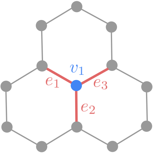
The next natural question is therefore: what is the interpretation of transposed boundary operators? Written in matrix form, \(\partial_i\) tells us which \((i-1)\)-chains are incident to a given \(i\)-chain. For instance, in a 2D cell complex, \(\partial_2(f)\) gives us all the edges incident to the face \(f\), and \(\partial_1(e)\) gives us the two vertices incident to the edge \(e\). Conversely, \(\partial_i^T\) tells us which \(i\)-chains are incident to a given \((i-1)\)-chain. For instance, \(\partial_2^T(e)\) gives us all the faces incident to the edge \(e\), and \(\partial_1^T(v)\) gives us all the edges incident to the vertex \(v\). For example, we have in the following figure \(\partial_1^T(v_1) = e_1 + e_2 + e_3\):
In fact, for cellulations of closed manifolds (i.e. compact manifolds without boundary), the cochain complex can be interpreted as the chain complex of the dual cellulation, after some reindexing. It is constructed by replacing all \(D\)-cells by vertices, all \((D-1)\)-cells by edges (connecting the vertices corresponding to the adjacent \(D\)-cells), all \((D-2)\)-cells by faces, and all \((D-i)\)-cells by \(i\)-cells in general. Applying this to a hexagonal cellulation of the torus, we get the following dual cellulation (blue):
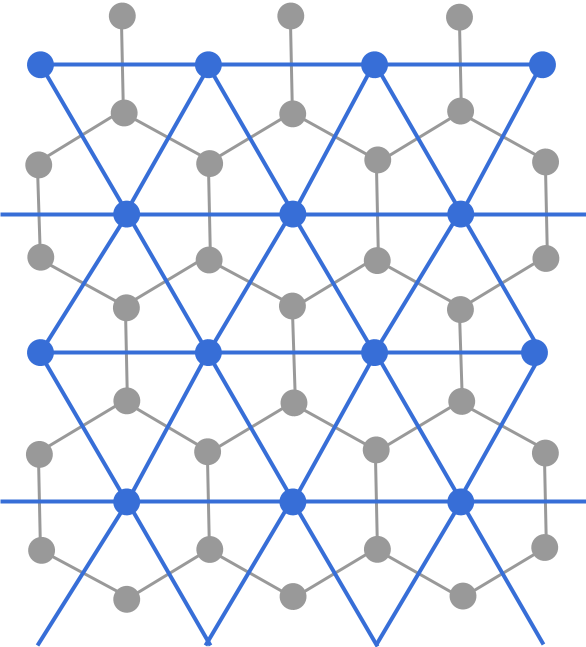
Schematically, if \(C^\star_j\) denotes the space of \(j\)-cells in the dual cellulation, the cochain complex can be identified with the chain complex of the dual cellulation as
\[\begin{array}{ccccccccc} C^0 & \overset{\delta^1}{\longrightarrow} & C^1 & \overset{\delta^2}{\longrightarrow} & \cdots & \overset{\delta^{D-1}}{\longrightarrow} & C^{D-1} & \overset{\delta^D}{\longrightarrow} & C^D \\ \cong & & \cong & & & & \cong & & \cong \\ C^\star_D & \overset{\partial^\star_D}{\longrightarrow} & C^\star_{D-1} & \overset{\partial^\star_{D-1}}{\longrightarrow} & \cdots & \overset{\partial^\star_2}{\longrightarrow} & C^\star_1 & \overset{\partial^\star_1}{\longrightarrow} & C^\star_0 . \end{array}\]The difference between the cochain complex and the dual complex is therefore just a matter of interpretation and indices: \(i\)-dimensional objects of the cochain complex are interpreted as \((D-i)\)-dimensional objects in the dual cell complex, but the spaces and maps are algebraically the same, up to the relabeling \(C^i \leftrightarrow C^\star_{D-i}\) and \(\delta^i \leftrightarrow \partial^\star_{D-i+1}\).
This gives us all the elements needed to define cohomology. The cohomology groups \(H^i(C_\bullet)\) of a chain complex \(C_\bullet\) are simply the homology groups of the cochain complex:
\[\begin{aligned} H^i(C_\bullet) &:= H_i(C^\bullet) \\ &= \ker(\delta^{i+1}) / \Im(\delta^{i}) \\ &\cong \ker(\partial_{i+1}^T) / \Im(\partial_{i}^T) \end{aligned}\]where the last line comes from the isomorphism between \(C^\bullet\) and \(\tilde{C}^\bullet\) that we saw earlier.
In the case of cell complexes, can we interpret the cohomology groups as the homology groups of the dual cellulation? Yes, as long as we make sure to use the right indices:
\[\begin{aligned} H^i(C_\bullet) \cong H_{D-i}(C^\star_\bullet). \end{aligned}\]Going back to quantum error correction, we can give cohomology a clear interpretation. Consider the length-2 chain complex associated to a CSS code with parity check matrices \(H_X\) and \(H_Z\),
\[\begin{aligned} \mathcal{S}_X &\xrightarrow{H_X^T} \mathcal{Q} \xrightarrow{H_Z} \mathcal{S}_Z \end{aligned}\]We saw that the first homology group, \(H_1(C_\bullet)=\ker(H_Z)/\Im(H_X^T)\), represents the \(X\) logical cosets: errors that commute with all \(Z\) stabilizers and are defined up to \(X\) stabilizers. Conversely, the cochain complex is given by
\[\begin{aligned} \mathcal{S}_Z &\xrightarrow{H_Z^T} \mathcal{Q} \xrightarrow{H_X} \mathcal{S}_X \end{aligned}\]and the first cohomology group by \(H^1(C_\bullet) = \ker(H_X) / \Im(H_Z^T)\). It can be interpreted as the set of \(Z\) logical cosets: errors that commute with all \(X\) stabilizers and are defined up to \(Z\) stabilizers. Therefore, when a CSS code comes from the cellulation of a manifold, its \(X\) logical operators are cycles of the original lattice while its \(Z\) logical operators are cycles of the dual lattice. This echoes what we already saw in the context of the surface code!
Relationships between homology and cohomology groups
Given a chain complex \(C_\bullet\), we can now extract a set of homology groups \(H_i(C_\bullet)\) and cohomology groups \(H^i(C_\bullet)\). But is there any relationship between them? For instance, is it possible to deduce the cohomology groups from the homology groups? Or the \(i\)th (co)homology group from the \(j\)th (co)homology group for some \(i\) and \(j\)?
The QEC intuition suggests that such a relationship should exist. The numbers of independent \(X\) and \(Z\) logicals are the same, and there is a basis \(\{\bar{X}_i,\bar{Z}_i\}\) such that \(\bar{X}_i\) and \(\bar{Z}_j\) intersect non-trivially mod \(2\) only for \(i=j\). Can we prove this rigorously from homological algebra?
The answer is yes, and we will see here two important theorems that relate homology and cohomology groups. The first one, called the universal coefficient theorem (UCT), shows that \(H_i(C_\bullet)\) and \(H^i(C_\bullet)\) are actually isomorphic if \(C_\bullet\) is a chain complex over \(\mathbb{Z}_2\), and gives bases for both that satisfy the intersection property mentioned above. The second one, Poincaré duality, applies to cellulations of manifolds and shows that \(H_i(C_\bullet)\) and \(H^{D-i}(C_\bullet)\) are isomorphic. Together with the UCT, it also means that \(H_i(C_\bullet)\) and \(H_{D-i}(C_\bullet)\) are isomorphic, so for cell complexes coming from closed manifolds, we only ever need to calculate half of the homology groups.
Universal coefficient theorem
Considering a chain complex such that each \(C_i\) is a finite-dimensional vector space over \(\mathbb{Z}_2\)2, the universal coefficient theorem can be formulated as follows:
Equivalently, using the isomorphism between chains and cochains, we can write (with a slight abuse of notation) \(\phi([f])([x]) = f^T x\). The proof of the universal coefficient theorem for vector spaces is a fun linear algebra exercise:
Another way to phrase the UCT is in terms of the intersection form. After identifying cochains with column vectors, define
\[\begin{aligned} \Phi: C^i \times C_i &\longrightarrow \mathbb{Z}_2 \\ (f,x) &\longmapsto f^T x . \end{aligned}\]This pairing counts the number of cells where the cocycle \(f\) and the cycle \(x\) overlap, modulo \(2\). From the UCT, we can deduce the following property of the intersection form:
In other words, whether a given cycle and cocycle intersect on an even or odd number of elements only depends on their homology and cohomology classes, not on the specific representatives chosen.
This leads to the statement we wanted on bases of homology and cohomology groups:
Applied to the CSS chain complex, this tells us precisely that there is a basis of \(X\) logical operators \(\{\bar{X}_i\}\) and a basis of \(Z\) logical operators \(\{\bar{Z}_i\}\) such that \(\bar{X}_i\) and \(\bar{Z}_j\) intersect an odd number of times only for \(i=j\) (for any representatives).
There are simpler ways to prove this fact (for instance using symplectic spaces, see Proposition 2.2.7 of my thesis), but I think it’s fun to also see it as a consequence of the universal coefficient theorem.
The following exercise contains the proof of the two corollaries above.
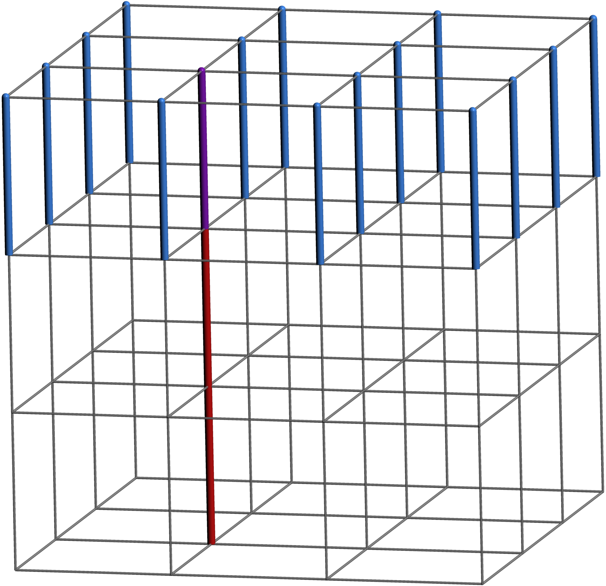
Here is an example of UCT homology-cohomology pairing for a 3D torus, where I highlighted a \(1\)-cycle in red and a corresponding \(1\)-cocycle in blue. These can be seen as \(X\) and \(Z\) logicals in a 3D toric code.
Before finishing this section, let’s briefly answer a question you might have been wondering this whole time: why is this theorem called “universal coefficient theorem”? We didn’t really talk about any kind of coefficient universality in our formulation of the UCT. The short answer is that the full theorem describes what happens when we change the coefficient group.
Consider a chain complex \(C_\bullet\) over the ring of integers \(\mathbb{Z}\), such that each \(C_i\) and each \(H_i(C_\bullet)\) is free (i.e. have a well-defined basis). We can then define the cohomology with coefficients in an abelian group \(G\), \(H^i(C_\bullet;G)\), as the homology of the cochain complex \(\text{Hom}(C_\bullet,G)\). The (more general) UCT then gives us the following isomorphism:
\[\begin{aligned} H^i(C_\bullet;G) \cong \text{Hom}(H_i(C_\bullet),G) \end{aligned}\]This means that we can obtain cohomology with coefficients in any group \(G\) from the homology groups of the chain complex over \(\mathbb{Z}\), making \(\mathbb{Z}\) a “universal” coefficient ring. More generally, if the homology groups are not free, the UCT also gives us a way to compute cohomology groups with coefficients in \(G\) from homology groups with coefficients in \(\mathbb{Z}\), but the relation is more complicated and involves homology groups at different levels.
Poincaré duality
In the case of the cellulation of a closed manifold, we can go one step further and relate the homology and cohomology groups of different indices. This is known as Poincaré duality.
Using the UCT, this also implies that \(H_i(C_\bullet) \cong H_{D-i}(C_\bullet)\), or, in terms of Betti numbers, \(b_i = b_{D-i}\).
Why is Poincaré duality true? Remember that \(H^i(C_\bullet)\) can be interpreted as the homology group of the dual cellulation, \(H_{D-i}(C^\star_\bullet)\). But all cellulations of a manifold \(\mathcal{M}\) have the same homology groups, so in particular \(H_{D-i}(C^\star_\bullet) \cong H_{D-i}(C_\bullet)=H_i(\mathcal{M})\).
However, this argument does not provide us with a very concrete isomorphism between \(i\)-cochains and \((D-i)\)-chains. Another formulation of Poincaré duality uses the notion of cap product to derive a very concrete way to go from \(i\)-cochains to \((D-i)\)-chains. You can find that version of the theorem in Hatcher, Section 3.3.
For a 3D torus, Poincaré duality maps for instance any \(1\)-cycle (e.g. a string of edges with no boundary) to a \(2\)-cocycle (e.g. a string of parallel faces with no coboundary). Here is an illustration of such a \(1\)-cycle (red) and a Poincaré-dual \(2\)-cocycle (blue):
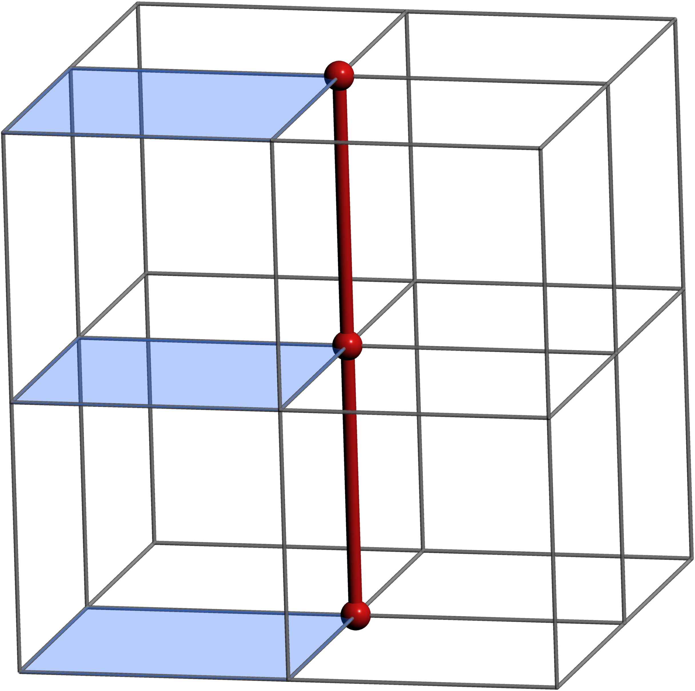
From a QEC perspective, Poincaré duality tells us for instance directly that any surface code defined on a cellulation of the 3-torus has the same number of logical qubits, no matter whether we define the code using \(C_2 \rightarrow C_1 \rightarrow C_0\) (which has \(k=b_1\)) or \(C_3 \rightarrow C_2 \rightarrow C_1\) (which has \(k=b_2\)).
More generally, we saw in the previous post that the \(D\)-torus has Betti numbers \(b_i=\binom{D}{i}\). Poincaré duality can be seen here from the symmetry of the binomial coefficients: \(\binom{D}{i} = \binom{D}{D-i}\).
Conclusion
We now have the missing half of the homological picture of QEC introduced in the previous post! Homology describes cycles modulo boundaries, which naturally captures one type of logical operator in a CSS code. Cohomology gives the dual story, capturing the other type through cocycles modulo coboundaries, or for closed manifolds, homology of the dual cellulation. The universal coefficient theorem tells us that, over \(\mathbb{Z}_2\), the intersection between cycles and cocycles only depend on their homology and cohomology classes, capturing the intersection property of logical operators in a CSS code. For cellulations of closed manifolds, Poincaré duality provides an isomorphism between homology and cohomology groups of complementary dimensions. Moving between the primal and the dual lattice, or between chain and cochain complexes, is often a very useful trick in QEC. For instance, color codes (and its generalizations) are defined from a lattice whose dual is a (colorable) simplicial complex, and it’s often easier to prove properties of the primal lattice by looking at the dual simplicial complex instead. But this will be the subject of another post!
There is much more to say about cohomology, and more generally about homological algebra, that is relevant for QEC. For instance, we can define a notion of cup product between cohomology classes, which can be used to find short-depth diagonal logical gates (including non-Clifford gates) in some CSS codes. We can define chain maps to relate different CSS codes or fault-tolerant protocols, or to find logical gates. Another concept, the mapping cone can allow us to design lattice surgery protocols or reduce the weight of stabilizers in a code. I hope to expand this series to cover all those concepts in the future! In the meantime, all this new knowledge should (hopefully) already make your next encounter with homological algebra in QEC papers feel a little less intimidating!
Solution of the exercises
-
A morphism of chain complexes (also called chain map) is a collection of linear maps \(f_i: C_i \to D_i\) between two chain complexes \(C_\bullet\) and \(D_\bullet\) that commute with the boundary operators, i.e. such that \(\partial_i^D \circ f_i = f_{i-1} \circ \partial_i^C\) for every \(i\). A chain map is an isomorphism if each \(f_i\) is an isomorphism of vector spaces. In our case, the isomorphism between \(C^\bullet\) and \(\tilde{C}^\bullet\) is given by the collection of isomorphisms \(\psi: C^i \to C_i\) for every \(i\). ↩︎
-
As a reminder, chain complexes are usually defined for general \(R\)-modules (see Footnote 1 of the previous post), which only become vector spaces when \(R\) is a field (such as \(\mathbb{Z}_2\)). ↩︎